Ecologial Census

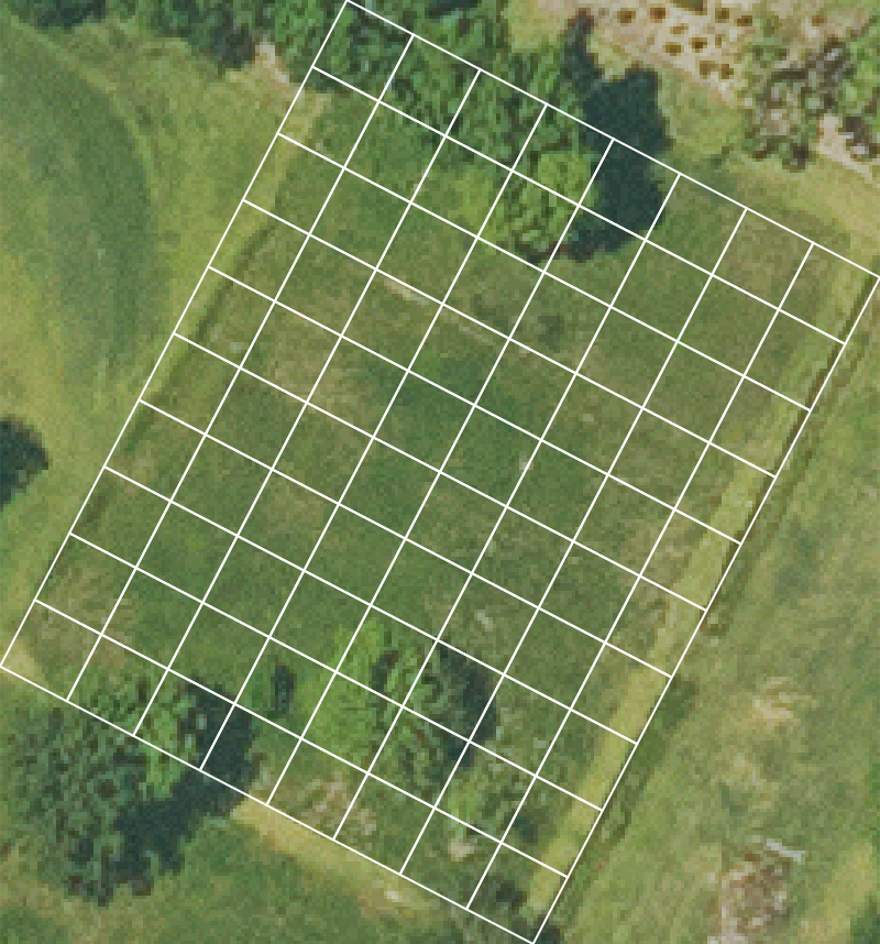
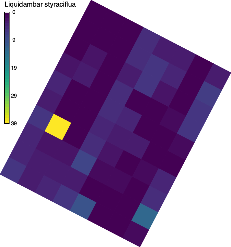
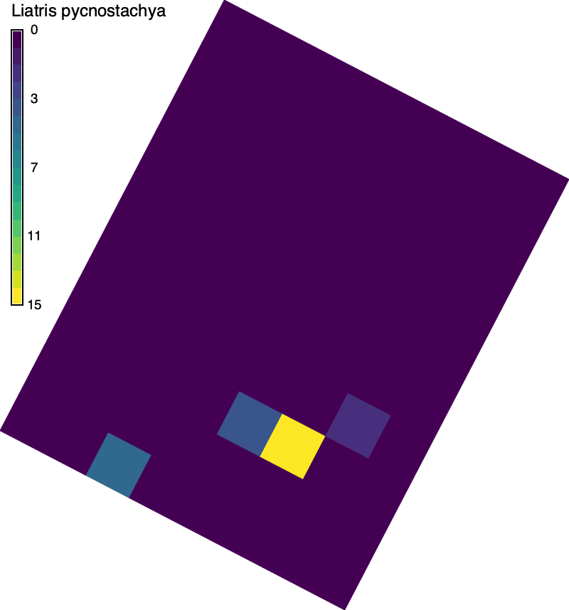
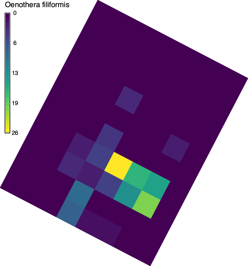
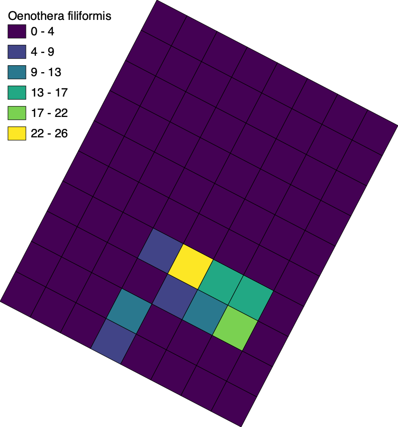
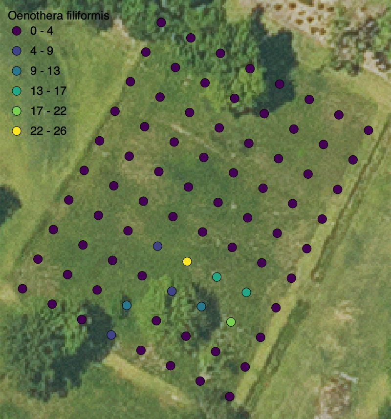
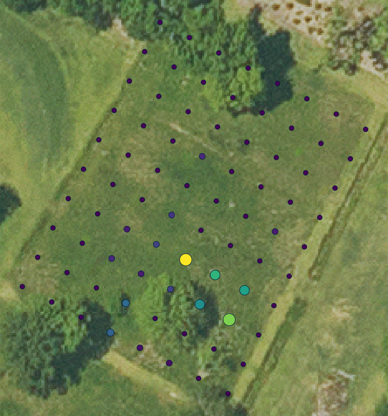
Mapping the distribution of Liquidambar styraciflua, Liatris pycnostachya, and Oenothera filiformis in the fourth quadrant of the meadow at the LSU Hilltop Arboretum. Download the project and table to get started.

Setup

# Import modules
import sys
import subprocess
from pathlib import Path
from contextlib import suppress

# Find GRASS Python packages
sys.path.append(
  subprocess.check_output(
    ["grass", "--config", "python_path"],
    text=True
    ).strip()
  )

# Import GRASS packages
import grass.script as gs
import grass.jupyter as gj
from grass.tools import Tools

# Create and initialize GRASS project
try:
    gj.init("hilltop")
except ValueError:
    with suppress(ValueError):
        gs.create_project("hilltop", epsg="2801")
        gj.init("hilltop")
tools = Tools(overwrite=True)

# Print projection
projection = tools.g_proj(format="shell", flags="p").keyval
print(projection.get("name"))

NAD83(HARN) / Louisiana South

Region

# Set region
tools.g_region(n=206040, s=205640, e=1023700, w=1022100, res=0.3)
tools.g_region(save="hilltop")

Census grid

# Set corner coordinate
coordinates="1022943, 205903"

# Create grid
tools.v_mkgrid(map="grid", grid=(10,8), position="coor", coordinates=coordinates, box=(6,6), angle=-27.5, type="area")

# Set region
tools.g_region(vector="grid")

# Visualize imagery
m = gj.Map(width=800, use_region=True)
m.d_rast(map="imagery")
m.d_vect(map="grid", color="white", fill="none", width=2)
m.show()

# Explore
m = gj.InteractiveMap(
    width=600,
    height=600,
    tiles="OpenStreetMap.Mapnik",
    use_region=True
    )
m.add_vector("grid")
m.show()

Census data

# Assign IDs
tools.v_db_update(map="grid", column="col", qcol="9 - col")
tools.v_db_update(map="grid", column="row", qcol="11 - row")
tools.v_db_addcolumn(map="grid", columns="id VARCHAR(10)")
tools.v_db_update(map="grid", column="id", query="row || CHAR(64 + col)")

# Set path to table
data = Path.cwd() / "data" / "census.csv"

# Import data
tools.db_in_ogr(input=data, output="census", overwrite=True)

# Make columns numeric
tools.db_execute(sql="ALTER TABLE grid ADD COLUMN ls INTEGER")
tools.db_execute(sql="ALTER TABLE grid ADD COLUMN lp INTEGER")
tools.db_execute(sql="ALTER TABLE grid ADD COLUMN of INTEGER")

# Join tables
tools.v_db_join(
    map="grid",
    column="id",
    other_table="census",
    other_column="ID",
    subset_columns=("ls", "lp", "of")
    )

# Export vector
tools.v_out_ogr(input="grid", output="census.gpkg", format="GPKG")

Liquidambar styraciflua

# Rasterize
tools.v_to_rast(
    input="grid",
    output="liquidambar_styraciflua",
    use="attr",
    attribute_column="ls"
    )

# Assign colors
tools.v_colors(map="grid", use="attr", column="ls", color="viridis")

# Visualize
m = gj.Map(width=800, use_region=True)
m.d_vect(map="grid")
m.d_legend(
    raster="liquidambar_styraciflua",
    color="black",
    title="Liquidambar styraciflua",
    title_fontsize=24,
    at=(50, 95, 2, 4),
    flags="s"
    )
m.show()

# Save image
m.save("liquidambar-styraciflua.png")

# Export raster
tools.r_out_gdal(
    input="grid",
    output="liquidambar-styraciflua.tif",
    format="GTiff"
    )

Liatris pycnostachya

# Rasterize
tools.v_to_rast(
    input="grid",
    output="liatris_pycnostachya",
    use="attr",
    attribute_column="lp"
    )

# Assign colors
tools.v_colors(map="grid", use="attr", column="lp", color="viridis")

# Visualize
m = gj.Map(width=800, use_region=True)
m.d_vect(map="grid")
m.d_legend(
    raster="liatris_pycnostachya",
    color="black",
    title="Liatris pycnostachya",
    title_fontsize=24,
    at=(50, 95, 2, 4),
    flags="s"
    )
m.show()

# Save image
m.save("liatris-pycnostachya.png")

# Export raster
tools.r_out_gdal(
    input="grid",
    output="liatris-pycnostachya.tif",
    format="GTiff"
    )

Oenothera filiformis

# Rasterize
tools.v_to_rast(
    input="grid",
    output="oenothera_filiformis",
    use="attr",
    attribute_column="of"
    )

# Assign colors
tools.v_colors(map="grid", use="attr", column="of", color="viridis")

# Visualize
m = gj.Map(width=800, use_region=True)
m.d_vect(map="grid")
m.d_legend(
    raster="oenothera_filiformis",
    color="black",
    title="Oenothera filiformis",
    title_fontsize=24,
    at=(50, 95, 2, 4),
    flags="s"
    )
m.show()

# Save image
m.save("oenothera-filiformis.png")

# Export raster
tools.r_out_gdal(
    input="grid",
    output="oenothera-filiformis.tif",
    format="GTiff"
    )

Color gradient

# Import libraries
import numpy as np
import matplotlib.cm as cm
import cmcrameri.cm as cmc
import cmasher as cmr

# # Set color map
# library = cmc
# colormap = "managua"
# gradient = getattr(library, colormap)

# Set color map
library = cm
colormap = "viridis"
gradient = getattr(library, colormap)

# Set number of classes
n = 6

# Generate color gradient
gradient = gradient(np.linspace(0, 1, n))
gradient = np.round(gradient[:, :3] * 255).astype(int)
gradient = [f"{r}:{g}:{b}" for r, g, b in gradient]

Thematic map

Tutorial: Thematic Maps

# Visualize
m = gj.Map(width=800, use_region=True)
m.d_vect_thematic(
    map="grid",
    column="of",
    legend_title="Oenothera filiformis",
    algorithm="int",
    nclasses=n,
    colors=gradient
    )
m.d_legend_vect(
    title_fontsize=48,
    fontsize=24,
    symbol_size=36,
    at=(2, 98)
    )
m.show()

Thematic dot map

# Extract centroids
tools.v_extract(input="grid", output="centroids", type="centroid")
tools.v_type(input="centroids", output="points", from_type="centroid", to_type="point")

# Visualize
m = gj.Map(width=800, use_region=True)
m.d_rast(map="imagery")
m.d_vect_thematic(
    map="points",
    column="of",
    legend_title="Oenothera filiformis",
    algorithm="int",
    nclasses=n,
    colors=gradient,
    icon="basic/point",
    size=36,
    )
m.d_legend_vect(
    title_fontsize=48,
    fontsize=24,
    symbol_size=36,
    at=(2, 98)
    )
m.show()

Proportional dot map

# Extract centroids
tools.v_extract(input="grid", output="centroids", type="centroid")
tools.v_type(input="centroids", output="points", from_type="centroid", to_type="point")

# Set specimen
specimen = "of"

# Set colors
tools.v_colors(map="points", use="attr", column=f"{specimen}", color="viridis")

# Visualize
m = gj.Map(width=800, use_region=True)
m.d_rast(map="imagery")
m.d_vect(map="points", size=20, icon="basic/point", where=f"{specimen} =0 OR {specimen} IS NULL")
m.d_vect(map="points", size=25, icon="basic/point", where=f"{specimen} > 0 AND {specimen} <= 5")
m.d_vect(map="points", size=30, icon="basic/point", where=f"{specimen} > 5 AND {specimen} <= 10")
m.d_vect(map="points", size=40, icon="basic/point", where=f"{specimen} > 10 AND {specimen} <= 20")
m.d_vect(map="points", size=50, icon="basic/point", where=f"{specimen} > 20 AND {specimen} <= 30")
m.d_vect(map="points", size=60, icon="basic/point", where=f"{specimen} > 30")
m.show()