Contents

• Flooding
• Flood Animation
• Flood Scenarios with the Raster Digitizer
• Depressions

Flooding

This tutorial will explore simple flood scenarios in GRASS GIS using the module r.lake the addon module r.lake.series, the raster digitizer, and the module r.fill.dir. The module r.lake creates a body of water by filling the terrain with water from a starting point. This algorithm represents the maximum possible extent of flooding for a given water level assuming that water spreads at an infinite speed from a source. It is an efficient way to represent the peak of a flood event. The addon module r.lake.series models flooding as a series of flood extents each with increasing water levels. It generates a time series of flood maps that can easily be animated. The raster digitizer, can be used to modify the topography in order to test different flood scenarios with r.lake or r.lake.series. The module r.fill.dir, an algorithm for generating depressionless digital elevation models, can be used fill depressions with water to represent local inundation in a rain event.

This tutorial uses the Governor’s Island Dataset for GRASS GIS. Download, extract, and move this geospatial dataset for Governor’s Island in New York City to your grassdata directory. Start GRASS GIS, set the GRASS GIS database directory to grassdata directory, select nyspf_governors_island as your location, and create a new mapset called flooding. Add the raster map elevation_2017 to the map display. Zoom in on the landforms in the southwest of the island. Either set the computation from the display using the various zoom options dropdown or run g.region and set the boundaries for the region. Save the region. To better visualize the topography generate a shaded relief map with the modules r.relief and r.shade.

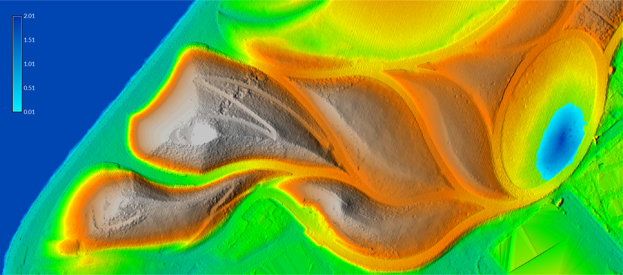
Model the maximum extent of a flood with a peak water level of 11.5 feet above sea level using r.lake. Set the input elevation raster to elevation_2017, the output lake raster to flooding, use the pointer to set the seed location to the lowest point in the oval lawn, approximately 978381.33268, 189447.513474, and then set the water level to 11.5 feet above sea level. This will flood the oval lawn right up to the edge of the pathway that circles it. Any higher water level and the flood would breach the pathway and spill over into the land below.

d.rast map=elevation_2017
g.region n=189850 s=189100 e=978550 w=976850 save=landforms
r.relief input=elevation_2017 output=relief zscale=2 units=survey --overwrite
r.shade shade=relief_2017 color=elevation output=shaded_relief brighten=30 --overwrite
r.lake elevation=elevation_2017 water_level=11.5 lake=flooding coordinates=978381.33268,189447.513474
d.legend raster=flooding at=60,95,2,3.5 font=Lato-Regular fontsize=14

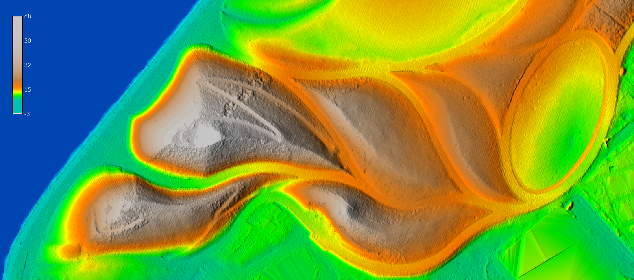
The module r.lake can also be used to model sea level on a digital elevation model. First try removing any raster masks with r.mask with the -r flag. Then use the raster map calculator r.mapcalc to add the sea floor to the digital elevation model. Write an map algebra expression with an if, then, else statement to generate the topobathy by replace null cells in the digital elevation model with the lowest elevation value present, i.e. 3 feet below sea level. If cells in the digital elevation model are null, then write -3, else write the existing elevation values. Then run r.lake with a seed location in the sea such as 976989.514944, 189704.054385 and a water level of 0. Use d.legend to add a raster legend with the font color set to white.

r.mask -r
r.mapcalc expression="topobathy = if(isnull(elevation_2017),-3,elevation_2017)"
r.lake elevation=topobathy water_level=0 lake=sea_level coordinates=976989.514944,189704.054385
d.legend raster=flooding at=60,95,2,3.5 font=Lato-Regular fontsize=14 color=white

Localized Flooding

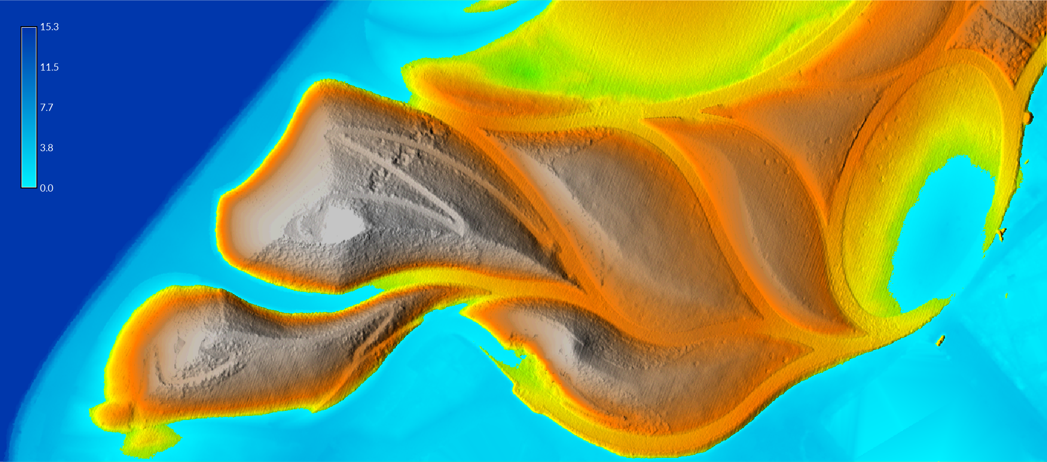
The landforms at Governor’s Island were designed to activate the site even when if it becomes inundated by storm surge or rising tides. The mounds, partly filled with rubble from old military buildings on the site, were built to rise above future high tides as sea level changes, maintaining access to this part of landscape. To model a flood that spreads across most of the landscape and breaches the pathway of the oval lawn, run r.lake with the water level set to 12 feet above sea level or greater. Set the input elevation raster to the topobathy and set the seed out at sea with the coordinates 976989.514944, 189704.054385.

r.lake elevation=topobathy water_level=12 lake=flooding coordinates=976989.514944,189704.054385 --overwrite

Coastal Flooding

Flood Animation

GRASS GIS has a temporal framework for analyzing and animating spatiotemporal phenomena. Raster and vector maps can be registered in space time raster and vector datasets in the temporal framework. In this tutorial we will simply use the temporal framework to animate a time series of flood maps. To learn more about the temporal framework read Gebbert & Pebesma, 2014 and Gebbert & Pebesma, 2017 and follow this tutorial: Spatio-temporal data handling and visualization in GRASS GIS.

Create a flood animation using the addon module r.lake.series and the animation tool g.gui.animation. First install the addon with g.extension. The addon module r.lake.series will generate a time series of flood maps based on a seed location, an initial water level, a final water level, a water level increment, and optionally a time step. Set the input elevation raster to topobathy, the output space time raster dataset to flooding, the starting water level to 9.8 feet, the end water level to 12 feet, the water level step to 0.1 feet, and the seed coordinates to 976989.514944, 189704.054385. Optionally set the time step with the time_step and time_unit parameters. The output will be a series of raster maps registered in a space time raster dataset using the temporal framework. Use the animation tool g.gui.animation to animate this space time raster dataset. Start the animation tool with the space time raster dataset to flooding. Then edit the animation to add the shaded relief map and then arrange the layers so that flooding is on top. Export the animation as an animated gif.

g.extension extension=r.lake.series
r.lake.series elevation=topobathy output=flooding start_water_level=6 end_water_level=14 water_level_step=0.1 coordinates=976989.514944,189704.054385
g.gui.animation strds=flooding

Flooding Animation

Flood Scenarios with the Raster Digitizer

Explore scenarios for storing storm water using the raster digitizer with r.lake. GRASS’ raster digitizer can be used to draw new raster maps or edit existing rasters. To create new conditions for a scenario use the raster digitizer to draw a check dam around the southeastern rim of the oval lawn on the digital elevation model. The check dam should temporarily hold storm water on the oval lawn during rain events, providing approximately 100,000 cubic feet of storm water storage capacity, while also serving as a seating element.

In the map display toolbar switch modes from 2D View to the raster digitizer. The digitizer toolbar will open in the map display. In the raster digitizer toolbar use the dropdown menu to create a new raster map named elevation, set the background raster map to elevation_2017, and set the raster type to FCELL for floating point values. This will create a copy of the digital elevation model that can be edited with the digitizer tools. Be sure to then select the new map in the dropdown menu. Use the digitizer’s line tool to draw a check dam around the oval lawn. Set the cell value to 14 feet above sea level and the line width to 2 cells. Once the line has been drawn save the raster map and exit the digitizer.

Digital Elevation Model with Check Dam

To better visualize the modified digital elevation compute shaded relief with r.relief and r.shade. Then model a flood event with r.lake. Set the input elevation raster to the modified elevation map, the output raster to flooding, and water level to 14, and the seed location to the lowest point in the oval lawn. Use the module r.volume to calculate the flood storage capacity of the oval lawn with a check dam in cubic feet.

r.relief input=elevation output=relief zscale=2 units=survey --overwrite
r.shade shade=relief color=elevation output=shaded_relief brighten=30 --overwrite
r.lake elevation=elevation water_level=14 lake=flooding coordinates=978381.33268,189447.513474 --overwrite
d.legend raster=flooding at=60,95,2,3.5 font=Lato-Regular fontsize=14 color=white
r.volume input=flooding

Flooding with Check Dam

Depressions

Since water will collect in low points in topography, these depressions can be used to represent ponding during rain events. The module r.fill.dir - an algorithm for identifying and filling depressions - can be used to model water collecting in depressions to form ponds. There is substantial noise in the lidar based digital elevation model that will register as tiny depressions. Use focal statistics to smooth the digital elevation model and eliminate the noise. Run the module r.neighbors with a 15 cell circular neighborhood using average operation. Then run r.fill.dir with the input elevation raster set to the smoothed digital elevation model. This will generate a depressionless digital elevation model. Then use the raster map calculator r.mapcalc with the following map algebra expression to extract the depressions. If the difference between the depressionless and smoothed digital elevation models is greater than a filter value, then write the difference, else write null values. For this example use a filter value of 0.3 feet. Then set the water color table for the map of depressions with r.colors and add a legend with d.legend.

r.neighbors -c input=elevation_2017@flooding output=smoothed_elevation method=average size=15
r.fill.dir input=smoothed_elevation output=depressionless_elevation direction=flow_direction
r.mapcalc expression="depressions = if(depressionless_elevation - smoothed_elevation  > 0.3, depressionless_elevation - smoothed_elevation, null())"
r.colors map=depressions color=water
d.legend raster=depressions at=60,95,2,3.5 font=Lato-Regular fontsize=14 color=white

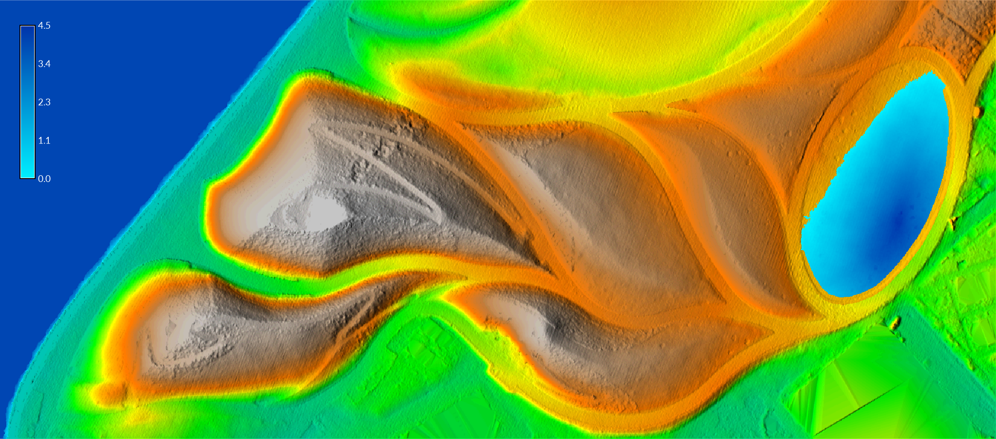
Depressions (ft)

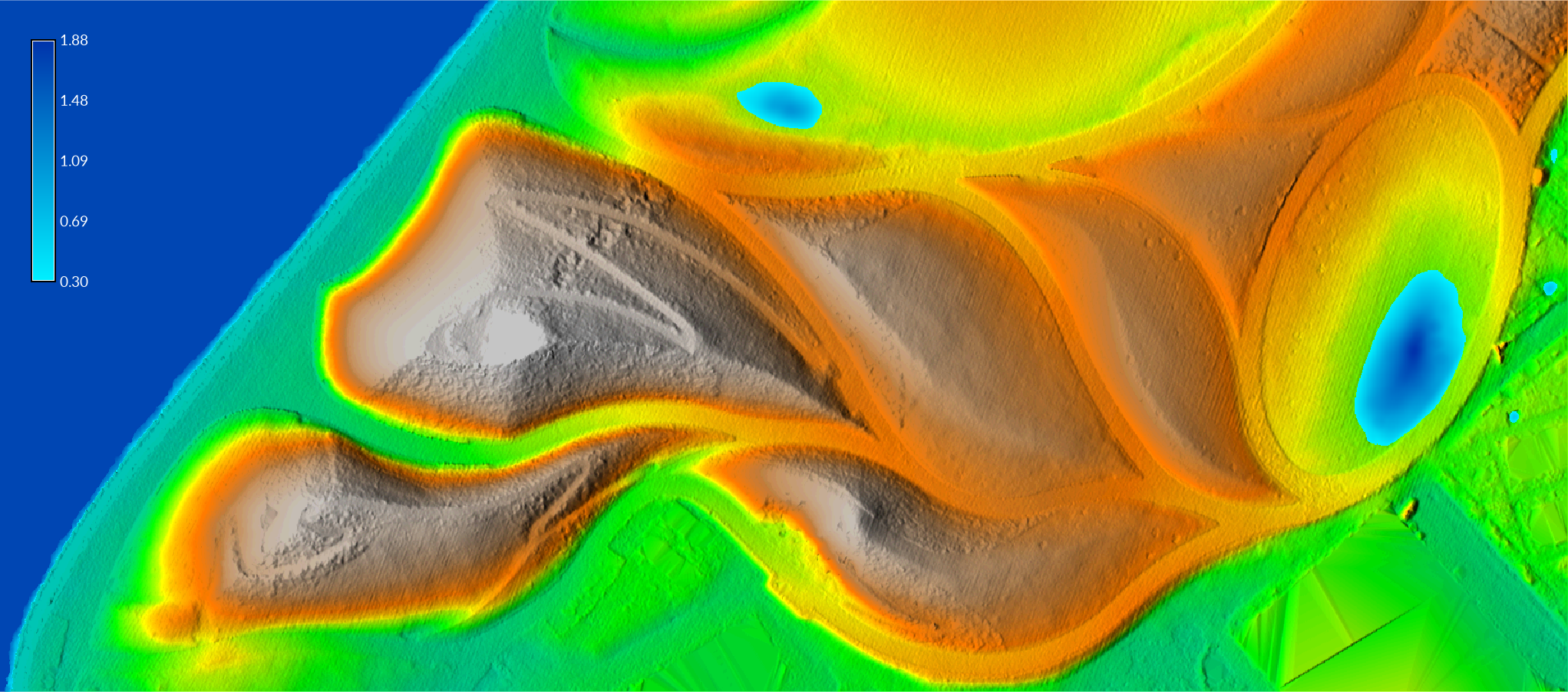Use either flow accumulation from r.watershed or shallow water flow depth from r.sim.water to map the flow of water into these depressions. For example add the map of water depth computed with r.sim.water in the hydrology tutorial. To display only concentrated flows of water run d.rast with the list of values to display starting at 0.05.

d.rast map=depth@hydrology values=0.05-99999

Since both the depression raster and the shallow water flow depth raster represent the depth of water they can be combined in order to share a color table and legend. Use map algebra with r.mapcalc to convert the depth raster from meters to feet and extract concentrated flows. If water depth is greater than 0.05, then write the product of water depth and the conversion factor 3.28, else write null values. Then use map algebra to overlay the rasters. If the depression raster is null, then write the depth raster, else write the depression raster. Set the water color table with r.colors and optionally apply histogram equalization with -e flag. Finally add a legend with d.legend.

r.mapcalc expression="depth = if(depth@hydrology > 0.05, depth@hydrology * 3.28, null())"
r.mapcalc expression="combined_depth = if(isnull(depressions), depth, depressions)"
r.colors -e map=combined_depth color=water
d.legend raster=combined_depth at=60,95,2,3.5 font=Lato-Regular fontsize=14 color=white

Depth of Water Flow and Depressions (ft)
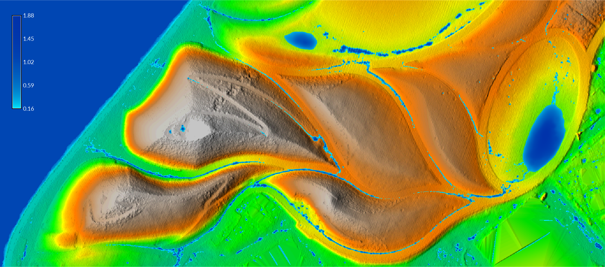