Hydrology in GRASS GIS
A tutorial on hydrological modeling and simulation in GRASS GIS.
Contents
- Hydrological Modeling
- Terrain Modeling
- Flow Accumulation
- Shallow Water Flow
- Shallow Water Flow with Landcover
- Shallow Water Flow with Vegetation Indices
- Shallow Water Flow Animation
- Manning’s Roughness Coefficients
Hydrological Modeling
This tutorial introduces hydrological modeling in GRASS GIS using r.watershed, r.sim.water, and r.lake. Learn more about hydrology in GRASS on the grasswiki page. GRASS GIS includes many modules and addons for hydrological modeling and analysis including:
- r.watershed
- r.lake
- r.lake.series
- r.sim.water
- r.stream.extract
- r.stream.distance
- r.stream.order
- r.filldir
- r.hydrodem
- r.terraflow
- ITZI
This tutorial uses the
Governor’s Island Dataset for GRASS GIS.
Download, extract, and move this geospatial dataset
for Governor’s Island in New York City
to your grassdata directory.
Start GRASS GIS,
set the GRASS GIS database directory to grassdata directory,
select nyspf_governors_island as your location,
and create a new mapset called hydrology.
Tested for GRASS-8.2.0-1.
Terrain Modeling
Zoom in on the landforms in the southwest of the island.
Either set the computation region from the display
using the various zoom options dropdown or
run g.region
and set the boundaries for the region. Save the region.
Then set a mask to the vector map shoreline with the module
r.mask.
The digital elevation model from lidar
has substantial noise that would impact hydrological simulations.
To reduce this noise
smooth the digital elevation model using the module
r.neighbors
with a moving window size of 5.
Optionally make the moving window circular with flag -c.
Visualize the relief of the terrain using direct illumination with r.relief. The light source can be set using the altitude and azimuth settings. Then drape the relief map over the smoothed digital elevation model with r.shade. Alternatively try visualizing relief using diffuse illumination from the skyview factor - the proportion of the sky visible given the surrounding relief. First install the addon module r.skyview with g.extension. Then compute the skyview factor with r.skyview from 16 directions. A composite of the shaded relief and skyview factor will combine direct and diffuse illumination to better visualize relief. Use r.shade to drape the shaded relief map over the skyview factor. Add a legend by running d.legend in the command console or using the add raster legend button under the add map elements dropdown menu in the graphical user interface.
![]()
g.region n=189850 s=189100 e=978550 w=976850 save=landforms
r.mask vector=shoreline
r.neighbors -c input=elevation_2017 output=elevation size=5
r.colors -e map=elevation color=elevation
r.relief input=elevation output=relief zscale=2 units=survey
r.shade shade=relief color=elevation output=shaded_relief brighten=40
g.extension extension=r.skyview
r.skyview input=elevation output=skyview ndir=16
r.shade shade=skyview color=shaded_relief output=composite_relief brighten=80
d.legend raster=elevation at=60,95,2,3.5 font=Lato-Regular fontsize=14
| Skyview Factor |
|---|
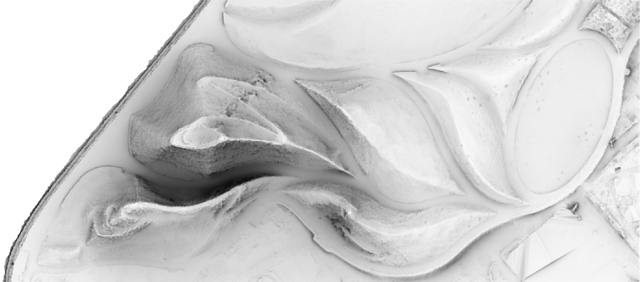 |
| Digital Elevation Model |
|---|
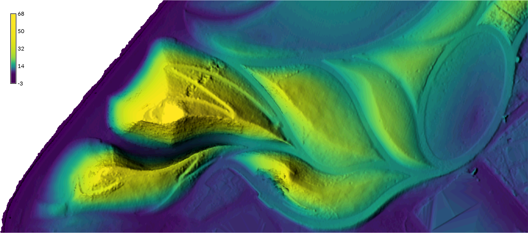 |
Flow Accumulation
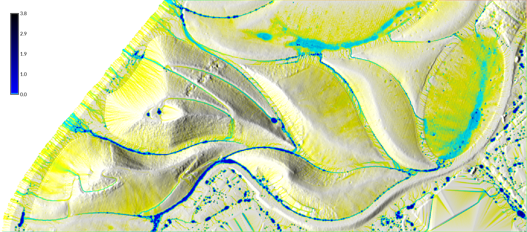
Flow accumulation - the number of cells that drain through each cell in an elevation raster - can represent the flow of water across a landscape. Compute flow accumulation with the module r.watershed. Then use r.shade to drape the flow accumulation map over the relief map.
r.watershed -a -b --overwrite elevation=elevation accumulation=flow_accumulation
r.shade shade=relief color=flow_accumulation output=shaded_accumulation brighten=40
d.legend -l raster=flow_accumulation at=60,95,2,3.5 font=Lato-Regular fontsize=14
| Flow Accumulation |
|---|
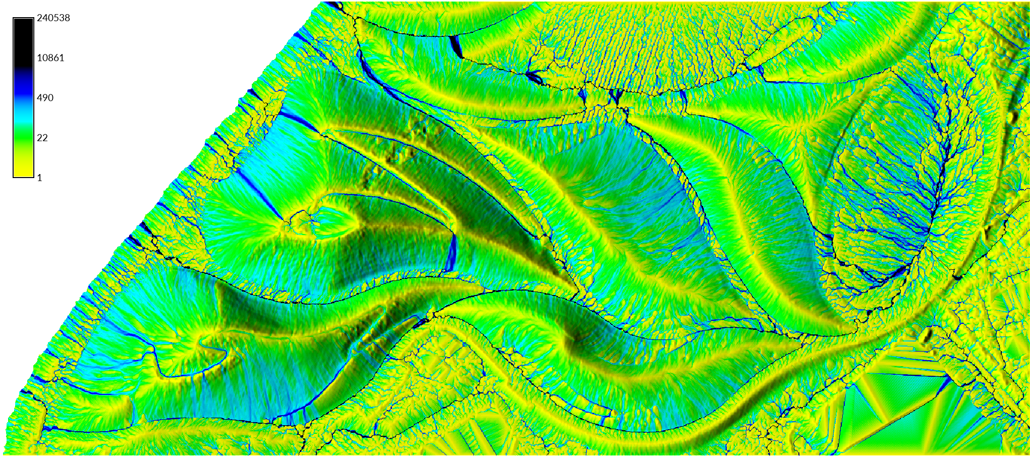 |
To visualize concentrated flow accumulation over the topography, use d.rast to set the range of values to display for the flow accumulation raster. To hide cells with low accumulation values, try setting the range from 100 to 1000000. Alternatively you could use map algebra with r.mapcalc to extract the concentrated flow values. Then layer this flow accumulation map on top of the shaded relief map.
d.rast map=composite_relief
d.rast map=flow_accumulation values=100-1000000
Shallow Water Flow
Simulate shallow flows of water over the landscape with
r.sim.water.
First compute the partial derivatives
dx and dy of the elevation raster
with
r.slope.aspect.
Then run
r.sim.water
for a 10 minute rainfall event with a rainfall rate of 150 \(mm/hr\).
Set the rainfall excess rate set to 150 \(mm/hr\),
the iteration time of 10 \(min\),
and the number of walkers to 10000.
Setting a higher number of walkers
will reduce noise in the solution
while increasing computation time.
Use r.sim.water
to generate maps of water depth \((m)\) and discharge \((m^3/s)\)
for a 10 minute storm.
Drape the depth or discharge map over the relief map
with r.shade.
r.slope.aspect elevation=elevation dx=dx dy=dy
r.sim.water elevation=elevation dx=dx dy=dy rain_value=150 nwalkers=10000 depth=depth discharge=discharge
r.shade shade=relief color=depth_with_landcover output=shaded_depth_with_landcover brighten=50
d.legend raster=depth_with_landcover at=60,95,2,3.5 font=Lato-Regular fontsize=14
| Shallow Water Flow Depth \((m)\) |
|---|
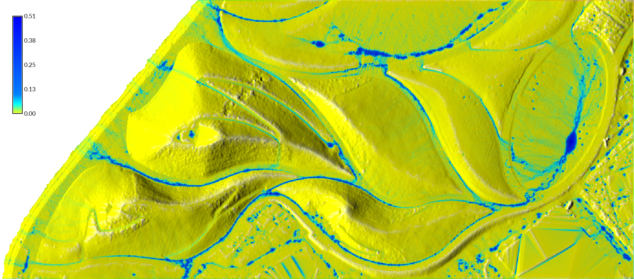 |
| Shallow Water Flow Discharge \((m^3/s)\) |
|---|
 |
To visualize concentrated flows over the topography, use d.rast to set the range of values to display for either the depth or discharge map To hide cells with low water depth values, try setting the range from 0.03-1.
d.rast map=composite_relief
d.rast map=depth values=0.03-1
Shallow Water Flow with Landcover
Simulate shallow overland flows of water
across different types of landcover with
r.sim.water.
Landcover can be derived from orthophotography
using unsupervised image classification,
supervised image classification,
or vegetation indices.
For simplicity’s sake this example uses
unsupervised classification.
First derive landcover classes from
the 2018 orthophotograph
with red, green, blue, and near infrared channels
using unsupervised image classification.
Create imagery groups and subgroups
using the module
i.group.
In the i.group
interface, name the new imagery group imagery_2018,
click add, select the PERMANENT mapset,
and use the pattern imagery_2018.
to add all the channels for the 2018 orthophotograph
to the imagery group.
Then check edit/create subgroup
to create a new subgroup also named imagery_2018
and select all maps in the group.
Use module
i.cluster
with to calculate spectral signatures for 3 landcover classes
from the imagery group.
Then use the module
i.maxlik
to classify spectral reflectance based on spectral signatures.
Recode the resulting map of landcover classes
as Manning’s roughness coefficients using
r.recode.
Grass should have a Manning’s n value of 0.368,
hardscape should be 0.0404,
and bare land should be 0.0113.
See the appendix at the end of this tutorial
for a list of suggested Manning’s n values.
For r.recode
create a rules file called mannings.txt
with the following lines
to recode class values to Manning’s n values.
1:1:0.368:0.368
2:2:0.0404:0.0404
3:3:0.0113:0.0113
Then simulate shallow water flow
with spatially variable surface roughness
using the module
r.sim.water.
Set the man parameter to your Manning’s roughness map.
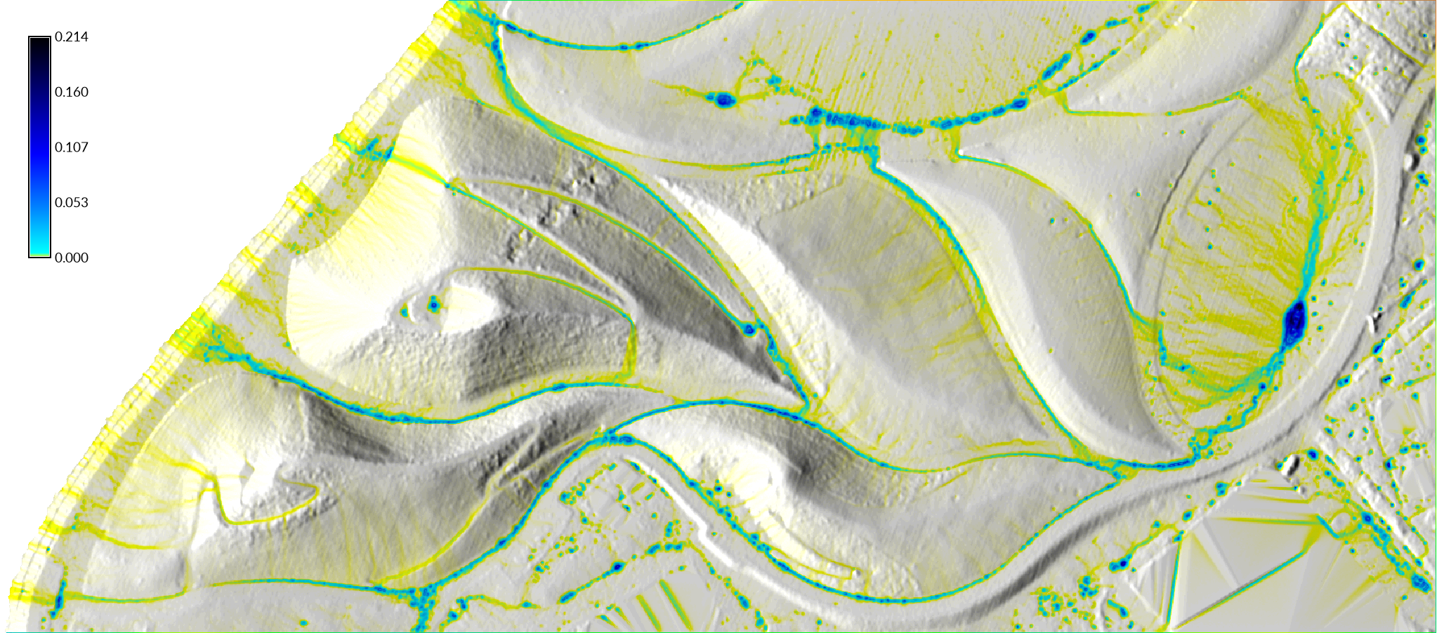
Drape the depth or discharge map over the relief map
with r.shade.
i.group group=imagery_2018 subgroup=imagery_2018 input=imagery_2018.1,imagery_2018.2,imagery_2018.3,imagery_2018.4
i.cluster group=imagery_2018 subgroup=imagery_2018 signaturefile=signature classes=3
i.maxlik group=imagery_2018 subgroup=imagery_2018 signaturefile=signature output=classification
r.recode input=classification output=mannings rules=mannings.txt
r.slope.aspect elevation=elevation dx=dx dy=dy
r.sim.water elevation=elevation dx=dx dy=dy rain_value=50 man=mannings nwalkers=10000 depth=depth_with_landcover discharge=discharge_with_landcover
r.shade shade=relief color=depth_with_landcover output=shaded_depth_with_landcover brighten=40
d.legend raster=depth_with_landcover at=60,95,2,3.5 font=Lato-Regular fontsize=14
| Manning’s Roughness Coefficient |
|---|
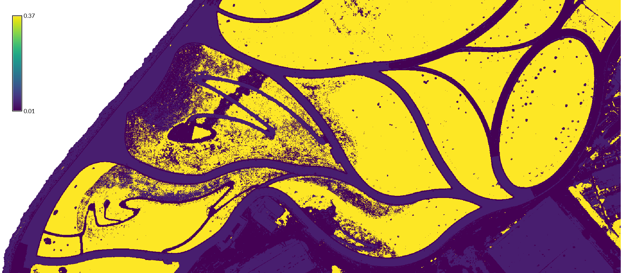 |
| Shallow Water Flow Depth \((m)\) with Landcover |
|---|
 |
| Shallow Water Flow Discharge \((m^3/s)\) with Landcover |
|---|
|
Shallow Water Flow with Vegetation Indices
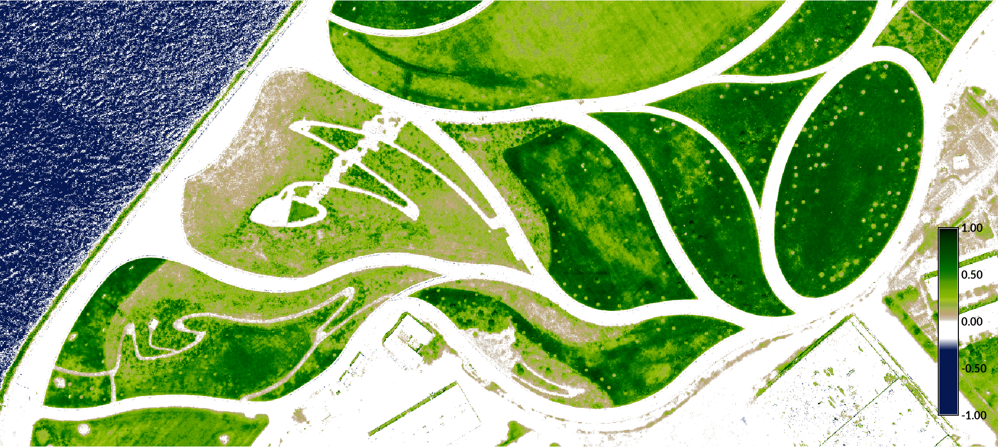
Vegetation indices such as Normalized Difference Vegetation Index (NDVI) can be used to classify landcover and derive Manning’s roughness. Derive roughness from NDVI to simulate shallow overland water flow. First use the module i.vi to compute NDVI with the red and near infrared channels of the 2018 orthophotograph.
\[NDVI = (NIR - red) / (NIR + red)\]Then recode the NDVI map
as Manning’s roughness coefficients using
r.recode.
To recode class values to Manning’s n values
either create a rules file called roughness.txt
with the following values or paste these values
into the r.recode dialog.
-1:-0.15:0.001:0.001
-0.15:0:0.0404:0.0404
0:0.2:0.2:0.2
0.2:1:0.368:0.368
Then simulate shallow water flow
with spatially variable surface roughness
using the module
r.sim.water.
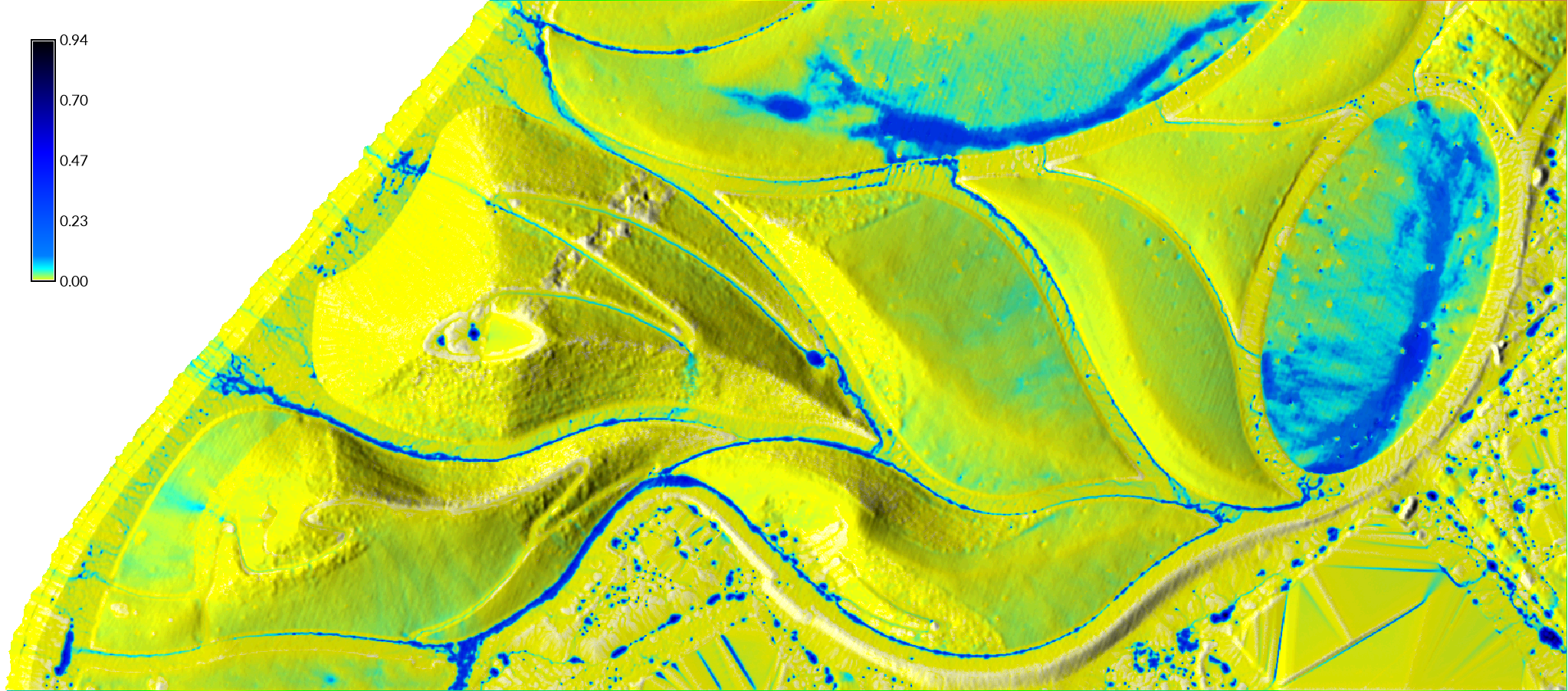
Set the man parameter to your Manning’s roughness map derived from NDVI.
Drape the depth or discharge map over the relief map
with r.shade.
i.vi output=ndvi red=imagery_2018.1 nir=imagery_2018.4
d.legend raster=ndvi at=5,45,94,96 font=Lato-Bold fontsize=16
r.recode input=ndvi output=roughness rules=roughness.txt
r.slope.aspect elevation=elevation dx=dx dy=dy
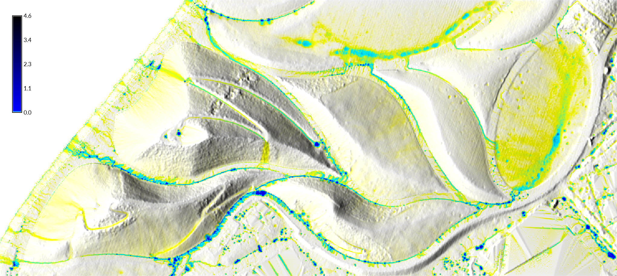
r.sim.water elevation=elevation dx=dx dy=dy rain_value=50 man=roughness nwalkers=10000 depth=depth_with_ndvi discharge=discharge_with_ndvi
r.shade shade=relief color=discharge_with_ndvi output=shaded_discharge_with_ndvi brighten=40
d.legend raster=discharge_with_ndvi at=60,95,2,3.5 font=Lato-Regular fontsize=14
| Normalized Difference Vegetation Index |
|---|
 |
| Shallow Water Flow Discharge \((m^3/s)\) with Landcover from NDVI |
|---|
 |
Shallow Water Flow Animation
Simulate and animate water flow over time.
First run
r.sim.water
with the -t flag to generate a time series of water depth or discharge maps.
Use g.list
with a search pattern of discharge.*
to generate a list of all of the discharge maps in the time series.
Copy the list, then run
g.gui.animation
to create an animation from the time series of discharge maps.
In the GRASS GIS Animation Tool
start by adding a new animation.
In the add new animation dialog
click the add space-time dataset layer button,
set the data type to multiple raster maps,
and then paste the list of discharge maps into the dialog box.
Optionally check the show raster legend box
and set the legend to the last map in the time series.
After the animation renders
adjust the size of the window and the animation speed
and then re-render
before exporting it as an animated gif.
r.sim.water -t --overwrite elevation=elevation dx=dx dy=dy depth=depth discharge=discharge nwalkers=10000 niterations=30 output_step=1
g.list type=raster pattern=discharge.* separator=comma
g.gui.animation raster=discharge.01,discharge.02,discharge.03,discharge.04,discharge.05,discharge.06,discharge.07,discharge.08,discharge.09,discharge.10,discharge.11,discharge.12,discharge.13,discharge.14,discharge.15,discharge.16,discharge.17,discharge.18,discharge.19,discharge.20,discharge.21,discharge.22,discharge.23,discharge.24,discharge.25,discharge.26,discharge.27,discharge.28,discharge.29,discharge.30
| Animated Shallow Water Flow Discharge |
|---|
 |
Optionally edit the animation to add the relief raster below the series of discharge maps. Set the opacity of the discharge maps to 80%.
Manning’s Roughness Coefficients
Manning’s n values are empirical coefficients for surface roughness. Based on literature I recommend the following n values for these types of landcover:
| NLCD Class | Landcover Category | Manning’s n value |
|---|---|---|
| 11 | Open Water | 0.001 |
| 21 | Developed, Open Space | 0.0404 |
| 22 | Developed, Low Intensity | 0.0678 |
| 23 | Developed, Medium Intensity | 0.0678 |
| 24 | Developed, High Intensity | 0.0404 |
| 31 | Barren Land | 0.0113 |
| 41 | Deciduous Forest | 0.36 |
| 42 | Evergreen Forest | 0.32 |
| 43 | Mixed Forest | 0.4 |
| 52 | Shrub/Scrub | 0.4 |
| 71 | Grassland/Herbaceuous | 0.368 |
| 81 | Pasture/Hay | 0.325 |
| 82 | Cultivated Crops | 0.325 |
| 90 | Woody Wetlands | 0.086 |
| 95 | Emergent Herbaceuous Wetlands | 0.1825 |