Contents

• Signed Distance Functions
• Docofossor Grid
• Elevation Rasters from GRASS
• Imagery from GRASS
• Importing Rasters into GRASS
• Lidar in GRASS

Signed Distance Functions

Docofossor, is a Grasshopper plugin for efficiently and iteratively modeling terrain using signed distance functions. Grasshopper is the visual programming interface for the 3D modeling program Rhino. To learn more about Grasshopper watch Grasshopper Basics with David Rutten, read the Grasshopper Primer, or study my course Generative Landscapes.

In Docofossor terrain is represented as a grid of elevation values (Z). Docofossor’s distance field data structure (df) – which is based on rasters – has a header that defines the properties of the grid and then a list of Z values. This grid of values can be transformed using signed distance functions, enabling an efficient, iterative process for terrain modeling in Grasshopper. To visualize the terrain data in Grasshopper the grid can be converted into either 3D points or a quadrilateral mesh.

To install on Windows first download Docofossor, right click on the zip archive to open properties and unblock it, then extract the zip archive, move the contents to your Grasshopper components library, and restart Rhino and Grasshopper. To learn more about Docofossor read the documentation and the paper Computational Terrain Modeling with Distance Functions for Large Scale Landscape Design.

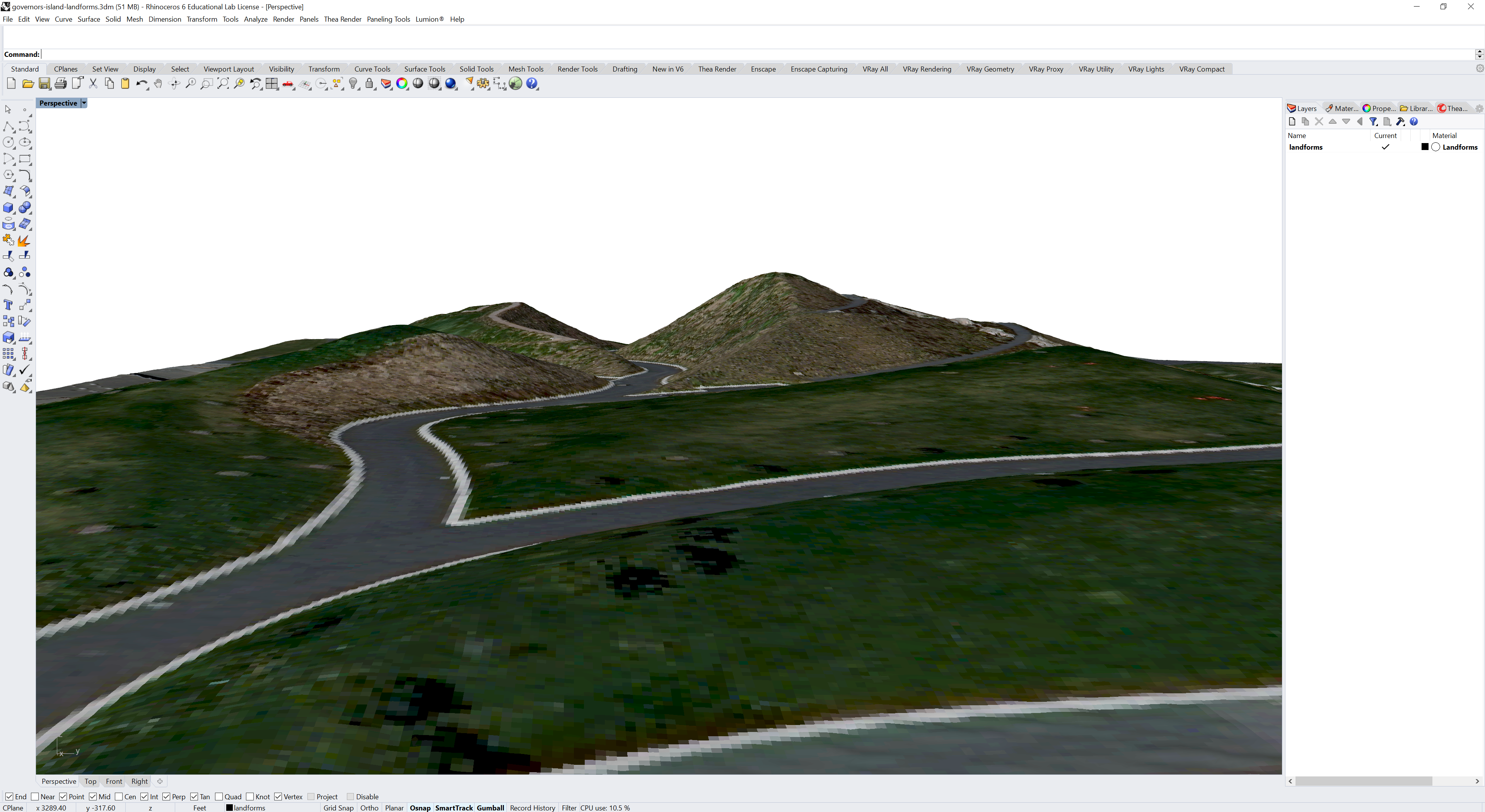
This tutorial uses Docofossor to model Governor’s Island, NYC from a gridded XYZ point cloud exported from GIS. For reference download the Grasshopper definition for this tutorial. To learn how to grade topography and calculate cut and fill with Docofossor watch my tutorials on Terrain Modeling, Terrain Analysis, and Grading Terrain.

Docofossor Grid

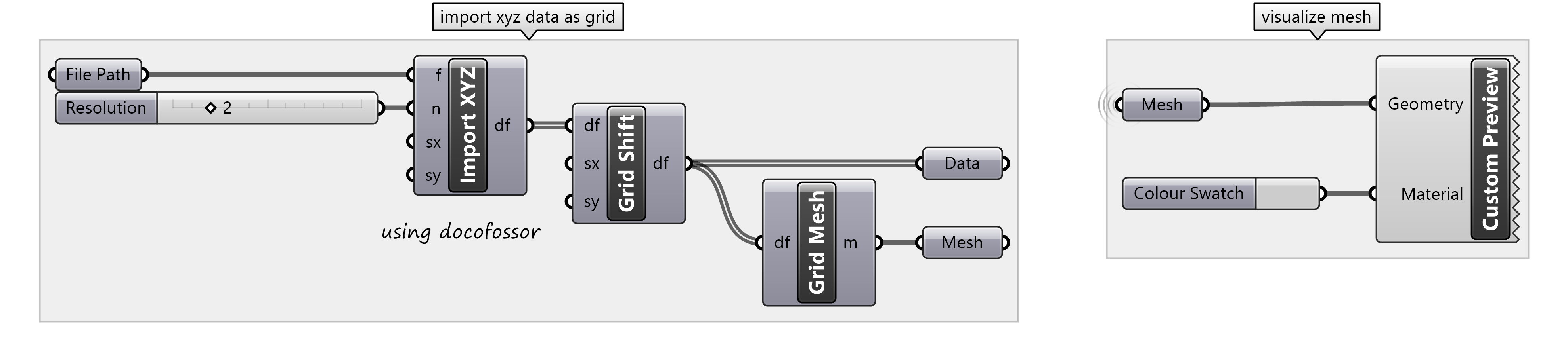
Download the gridded point cloud governors-island-landform.xyz for the landforms on Governor’s Island. In Grasshopper add the file path for this dataset to your canvas as a parameter. In the Params tab under Primitive select and add a File Path parameter. Right click on the parameter, choose select an existing file, and set the path to the downloaded .xyz data. In the Docofossor tab under IO add the dfImportXYZ component. Set dfImportXYZ’s input parameter f to the File Path parameter to import the point cloud as a Docofossor grid (df). Optionally add a skip parameter n to reduce the size of the point cloud.

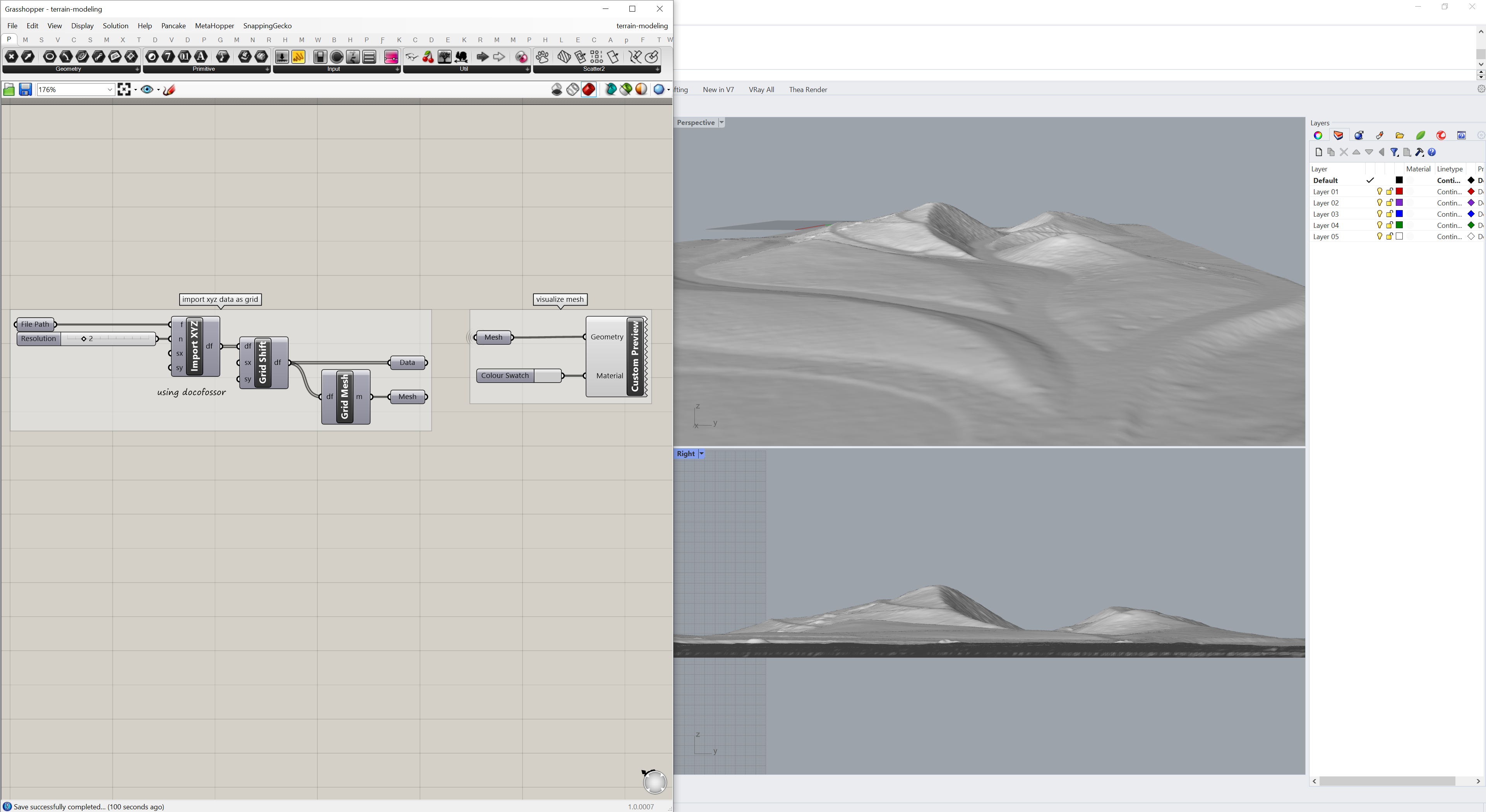
In the Docofossor tab under Grid add the dfGridShift component and set the grid as its input df to shift the grid to from its geographic coordinates to the XY origin of the local Cartesian coordinate system. In the Docofossor tab under Geometry add the dfGridMesh component to generate a quadrilateral mesh from the shifted grid. Connect a custom preview with a color swatch to output mesh to better visualize the landscape.

Since Docofossor expects points to be listed from left to right and from bottom to top, XYZ point clouds that are sorted differently - such as governors-island-landform.xyz - will be mirrored vertically on import. To fix this use the mirror component with the grid mesh as the input geometry and an XZ plane with its origin set to the center of the mesh as the input plane. Find the center of the mesh using the area component.

Elevation Rasters from GRASS

Docofossor requires XYZ point clouds with regular grid spacing. Rasters, which have regular grid spacing, can be exported as XYZ point clouds. To find raster elevation data, see my list of geospatial data sources. This section of the tutorial covers how to process raster data in GRASS GIS and export it for use in Rhino and Grasshopper.

Download and extract the Governor’s Island Dataset for GRASS GIS. Start GRASS in the nyspf_govenors_island location and create a new mapset named docofossor. Add the raster elevation_2017 from the PERMANENT mapset to the map display. First remove any raster mask with r.mask with the -r flag. Either zoom to the desired extent and set the computational region from the display under various zoom options or run g.region n=189850 s=189100 e=978550 w=976850 res=1 save=landforms in the command line. Docofossor does not handle grid cells with no data, so any null cells should be filled. Since the digital elevation model for Governor’s Island has null cells in the harbor around the island, these should be filled with elevation of sea level at low tide. First use univariate raster statistics with r.univar to find the minimum elevation value in the digital elevation model as a proxy for sea level at low tide. This may be between -3 to -4 feet depending on your region. Use map algebra with the raster calculator r.mapcalc to crop the digital elevation model to the computational region and fill the nulls cells. Write a map expression with a conditional if, then, else statement reading if cells in the map elevation_2017 are null, then write -3.39, else write values from elevation_2017. Export the resulting raster as an ASCII XYZ point cloud using the module r.out.xyz.

r.mask -r
g.region n=189850 s=189100 e=978550 w=976850 res=1 save=landforms
r.univar map=elevation_2017
r.mapcalc expression="elevation = if(isnull(elevation_2017), -3.39, elevation_2017)"
r.out.xyz input=elevation separator=comma

Imagery from GRASS

Orthoimagery - such as aerial photographs - can be mapped onto the surfaces or meshes in Rhino. To export raster imagery for Governor’s Island from GRASS first set the computational region, then crop the raster to the region with r.mapcalc, and then export the map as a .png in portable network graphics format with r.out.png.

g.region region=landforms
r.mapcalc expression="imagery = imagery_2018"
r.out.png --overwrite input=imagery output=D:\generative-design\grasshopper\data\govenors-island-imagery.png

To drape the aerial photograph over the terrain mesh in Rhino, first bake the mesh, then assign the picture as a material, and map the texture as plane to the bounding box of the mesh. In Grasshopper bake the mesh (from the mirror component) Disable the preview for all components and disable the custom preview. In Rhino set all viewports to rendered mode. Set a new material for the layer with the baked mesh by clicking on the layer’s material orb in the layer manager. Name the material Imagery, change the type to picture, and set the texture to govenors-island-imagery.png. Select the mesh and open the texture mapping tab in the object properties panel, and choose apply planar mapping. In the command line set the parameters for ApplyPlanarMapping. Set the plane to BoundingBox, the coordinate system to World, and the mapping to UV.

ApplyPlanarMapping

Importing Rasters into GRASS

Rasters can be imported into GRASS GIS with the module r.in.gdal. For imagery each channel will import as a separate raster map and will need to be combined together with r.composite. If rasters have been divided into tiles they can be patched together with r.patch.

Download the 2017 digital surface model tile hh_NYC_020.tif and 2018 orthoimagery tiles 977190 and 980190 for Governor’s Island. Note that FTP support is being disabled or removed from web browsers like Chome and Firefox due to security concerns. Either use a program such as FileZilla, the command line with curl, or enable FTP in your browser. For Chrome in chrome://flags/ turn on enable support for FTP URLs.

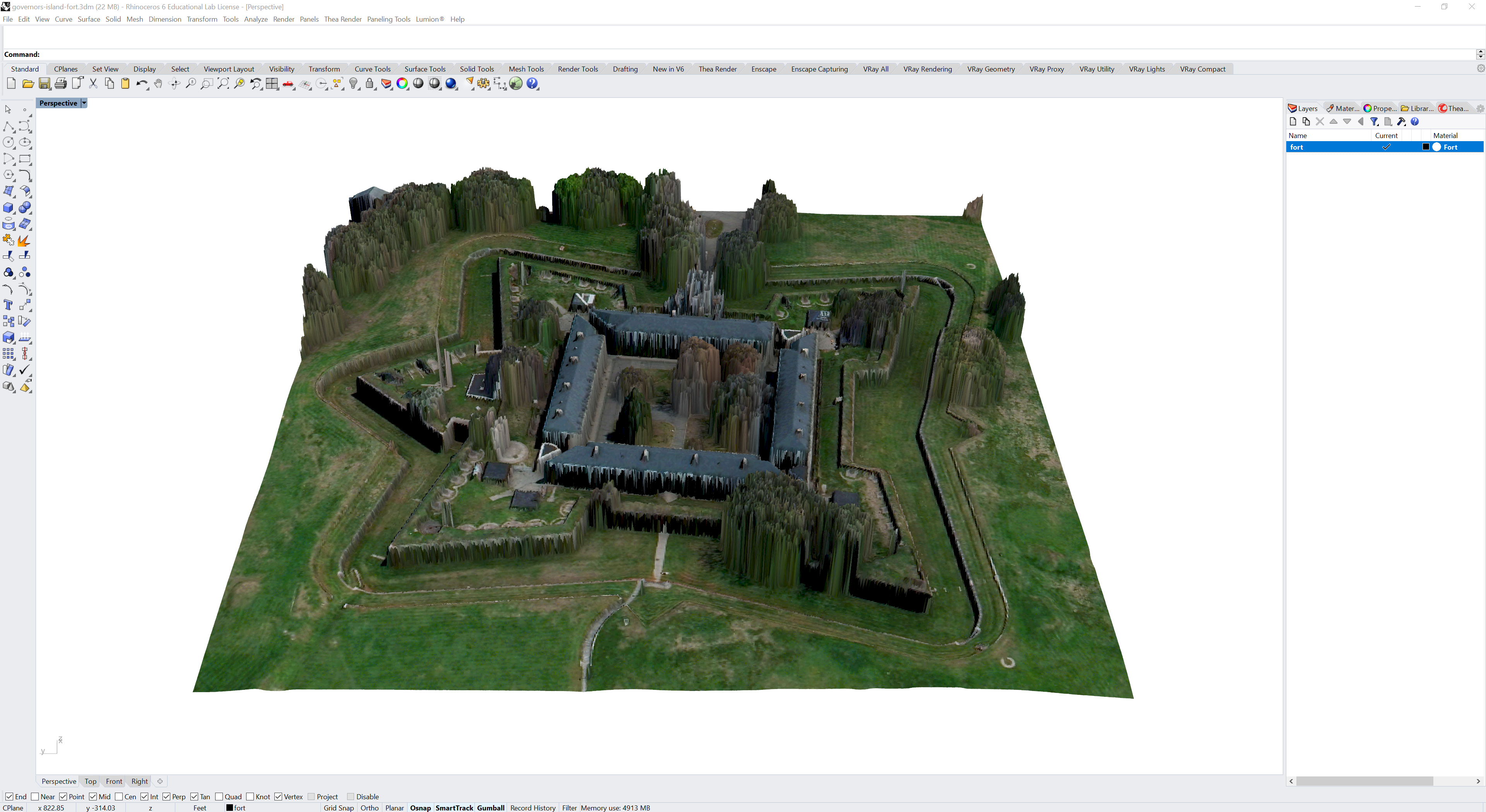
Start GRASS GIS and create a new location from georeferenced data. When creating the new location read the projection and datum terms from the digital surface model hh_NYC_020.tif. First import the digital surface model hh_NYC_020.tif with r.in.gdal. Set the computational region around the fort on the north of the island with g.region. Crop the digital surface model to the region with r.mapcalc and then export the resulting raster as an ASCII XYZ point cloud using r.out.xyz.

r.in.gdal input=hh_NYC_020.tif output=surface_2017
g.region n=191531 s=190812 w=979477 e=980181 res=1 save=fort
r.mapcalc expression="surface = surface_2017"
r.out.xyz input=surface output=governors-island-fort.xyz separator=comma

Import the imagery tiles 980190.jp2 and 980190.jp2 with r.in.gdal with the -r flag to limit the import to the computational region. Since the imagery has red, green, blue, and near-infrared channels, each tile of imagery will import as a series of four rasters. Composite each set together with r.composite and then patch the resulting rasters together with r.patch. Finally export the map as a .png in portable network graphics format with r.out.png.

r.in.gdal -r input=980190.jp2 output=imagery_2018_b
r.in.gdal -r input=977190.jp2 output=imagery_2018_a
r.composite red=imagery_2018_a.1 green=imagery_2018_a.2 blue=imagery_2018_a.3 output=imagery_2018_a
r.composite red=imagery_2018_b.1 green=imagery_2018_b.2 blue=imagery_2018_b.3 output=imagery_2018_b
r.patch input=imagery_2018_a,imagery_2018_b output=imagery_2018
r.out.png input=imagery_2018 output=governors-island-fort.png

Import the XYZ point cloud into Grasshopper as grid using Docofossor, generate a mesh from the grid, and bake the mesh to Rhino. Then map the imagery as a texture on the mesh.

Lidar in GRASS

Lidar, laser scanning, and photogrammetry generate unstructured point clouds. GRASS GIS can generate a raster surface from a point cloud either though binning or interpolation. To bin ASCII XYZ point clouds use the module r.in.xyz. To bin .las LASer point clouds use the module r.in.lidar. To interpolate a point cloud first import it as vector points with v.in.ascii if it is in ASCII XYZ format or with v.in.lidar if it is in LASer format. Use regularized spline with tension interpolation with v.surf.rst to approximate a raster surface from the vector points. Point clouds can also be gridded in CloudCompare with its Rasterize tool.