Using GRASS in QGIS
Contents
Rationale
While GRASS GRASS GIS has an extensive library with over 500 modules for spatial and temporal computation, QGIS is easier to use and has a handsome, modern user interface (UI). Since GRASS is integrated into QGIS, you can perform sophisticated spatial computations using GRASS modules and then compose beautiful maps in QGIS with the resulting data. To learn more read the GRASS GIS Integration section of the QGIS user manual.
There are two ways to use GRASS in QGIS. You can either load GRASS datasets in QGIS and then run modules using GRASS Tools. Or if you are working with data such as shapefiles, geotiffs, or geopackages, you can use GRASS algorithms in the Processing Toolbox.
The GRASS integration for QGIS can streamline workflows involving spatial computation and map making. With the integration users with more experience with QGIS can work entirely within QGIS, using the GRASS plugin when GRASS algorithms are needed. Users with more experience with GRASS, may prefer to run computations in GRASS and then load the GRASS datasets in QGIS to compose high quality maps for publication. Users with experience in GRASS who prefer the QGIS interface, can load their GRASS datasets in QGIS and run GRASS Tools in QGIS. This tutorial will demonstrate how to use GRASS Datasets and GRASS Tools inside of QGIS.
GRASS Plugin
Start QGIS Desktop with GRASS.
In the Plugins menu select Manage and Install Plugins.
Processing and
GRASS 7
are core plugins
so they are already installed, but need to be enabled.
Check the plugins to enable them.
GRASS Datasets
Download and extract the Governor’s Island Dataset for GRASS GIS.
The top level directory nyspf_governors_island
is a GRASS GIS location
for NAD_1983_StatePlane_New_York_Long_Island_FIPS_3104_Feet
in US Surveyor’s Feet.
Inside the location there is the PERMANENT mapset,
a license file, data record, readme file, workspace, color table,
category rules, and scripts for data processing.
Create a directory on your computer called grassdata.
This will be your GRASS GIS database
directory where you will store your GRASS locations and mapsets.
Move the location nyspf_govenors_island inside of your grassdata directory.
Browse to your grassdata directory in the browser panel
on the left side of the QGIS window.
Optionally right click and select
add as favorite to create a shortcut.
Expand your grassdata directory and
browse to find the GRASS location.
There will be a both
a directory with a icon
and a GRASS location with a icon
named nyspf_governors_island.
Expand the location
nyspf_governors_island
and select the PERMANENT mapset.
Expand the mapset
and add some data to your layer manager and map.
First try adding the
shoreline vector.
Expand the shoreline database
and double click on the
shoreline area to add it.
While the default coordinate reference system
for a new project is WGS 84 (EPSG 4326),
the project CRS will automatically switch
to that of the first layer added.
In this case the CRS will be
NAD83 / New York Long Island (ftUS) (EPSG 2263).
Now add a raster.
Double click on the
elevation_2017 to add this digital elevation model.
This raster will not render in the map display
with the default symbology settings.
You will need to specify a color ramp
and load values from the raster.
A color ramp for a digital elevation model
is called hypsometric tinting.
Double click on
elevation_2017
to open its layer properties menu.
In the symbology tab in the band rendering section,
first click load color map from band
to create a sequence of breakpoints
for a continuous color ramp,
then set the render type to Singleband psuedocolor,
and select a color ramp such as viridis
from the dropdown menu.
To select GRASS’s elevation color ramp instead,
choose create new color ramp
from the color ramp dropdown,
select the catalog: cpt-city type,
then under QGIS select grass color ramps,
and pick elevation.
See the cpt-city
topography collection for other great color ramps
such as wiki-schwarzwald-cont for
digital elevation models.
Save the color ramp to your favorites.
In the min / max value settings
set the accuracy to actual,
select a method such as min / max,
hit apply, then classify, and apply again.
In the resampling section
set zoomed in to bilinear or cubic.
Since a digital elevation model
represents a continuous gradient of data
you should use bilinear or cubic interpolation
for resampling instead of nearest neighbor
which is more appropriate for discrete data.
| Digital Elevation Model (DEM) |
|---|
 |
To blend a hillshade with the elevation color ramp,
first make a copy of the layer elevation_2017.
To do this right click on elevation_2017
and select duplicate layer.
Turn on the new layer, move it above the original layer,
and change its symbology.
Set the render type to hillshade
and the blending mode to soft light.
Adjust the settings.
For example try setting the z-factor to 2.
Try adjusting the azimuth
to cast the shade from a different angle.
Hit apply to visualize the changes.
Optionally rename the layer to shaded_elevation_2017.
| Digital Elevation Model (DEM) with Hillshading |
|---|
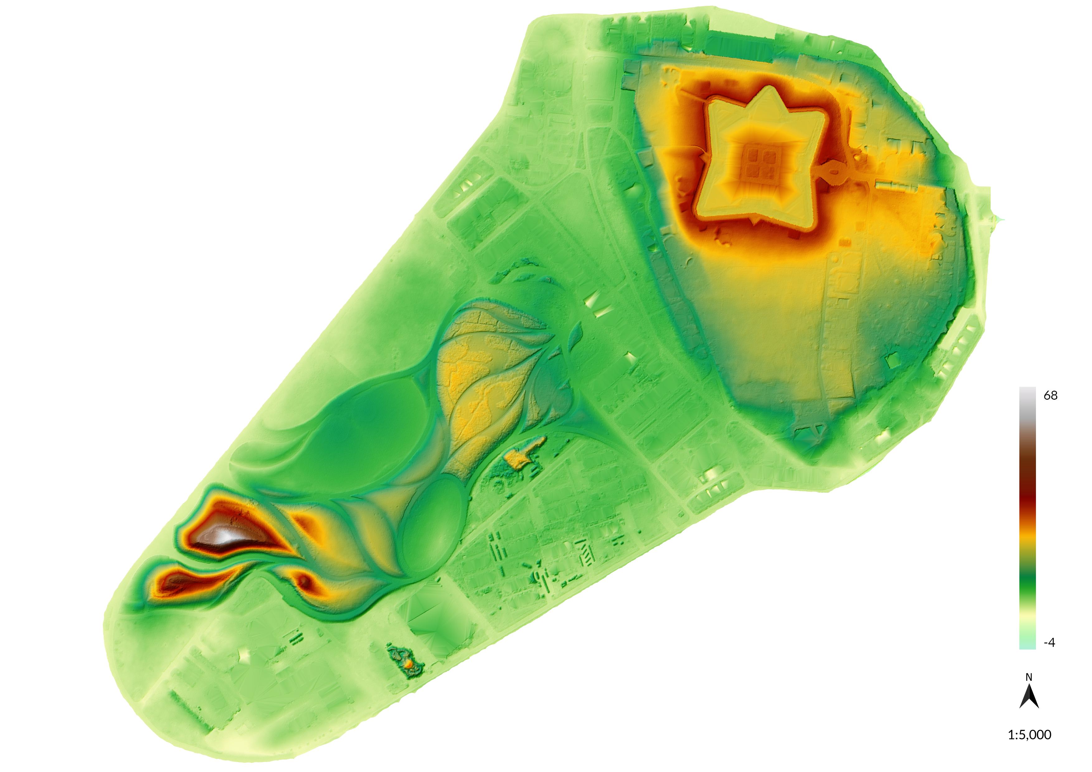 |
To add contour lines as a layer style,
first make another copy of the layer elevation_2017.
Turn on the new layer, move it above the original layer,
and change its symbology.
Set the render type to contours
and then adjust the settings.
Try setting the contour interval to 3 feet.
To reduce noise try setting input downscaling to 6 feet.
Try different blending modes
such as screen with 60% percent brightness.
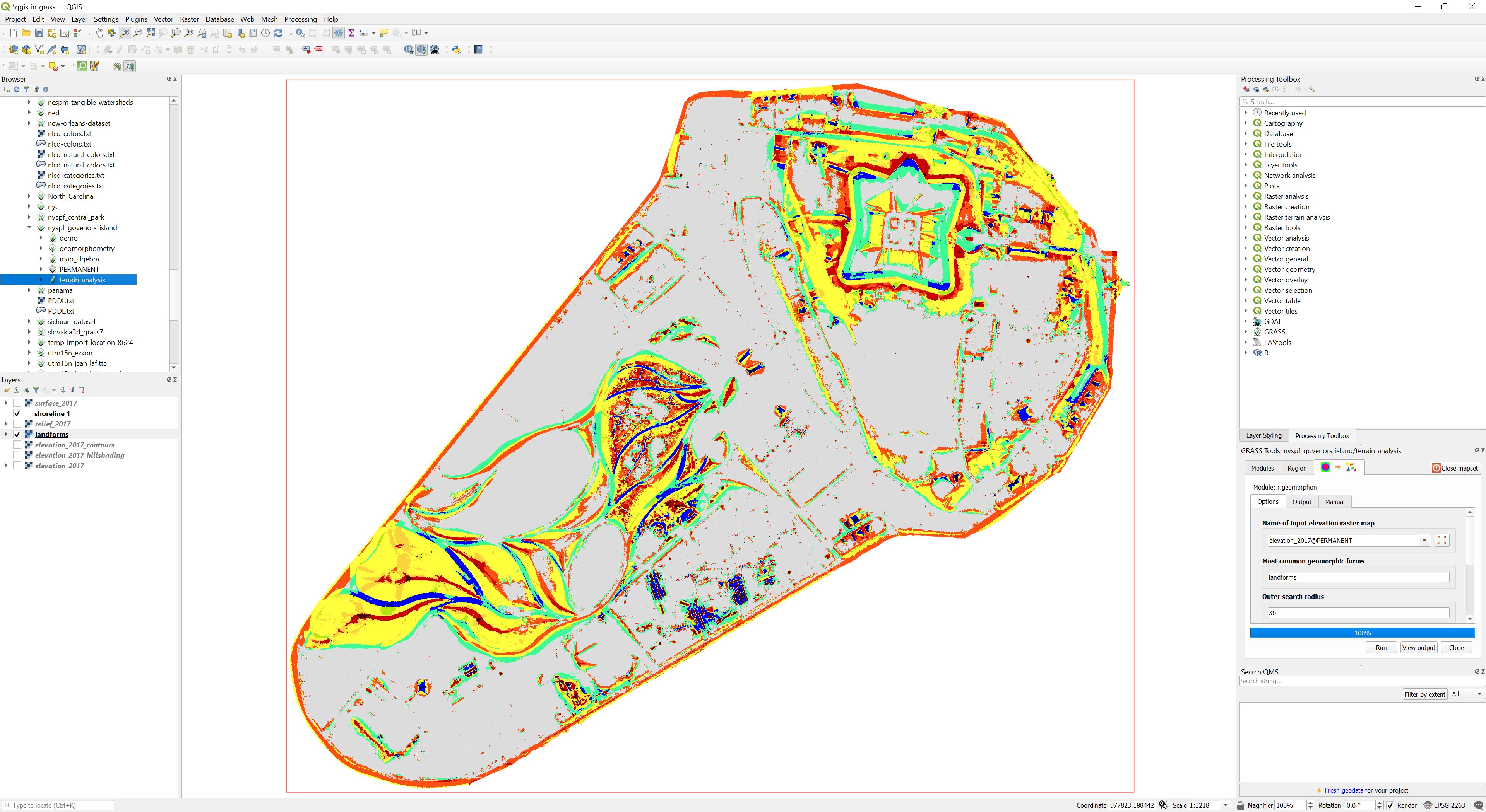
GRASS Tools
We will use GRASS Tools to set the computational region and then recognize and classify landforms with the GRASS module r.geomorphon.
In the browser expand the location
nyspf_governors_island.
Right click on the location
and select new mapset.
Name the mapset terrain_analysis.
Right click on the new mapset and select Open Mapset
to activate GRASS Tools.
GRASS Tools will open in a panel on the right.
The best practice for working with GRASS GIS
is to use the PERMANENT mapset for reference data
and use other mapsets for new data that you create.
This helps to preserve the original source data
and keep your project organized.
Whichever mapset you open,
you will still have access
to the maps in the PERMANENT mapset.
First set the computational region for raster operations.
In the region tab of GRASS Tools
click select the extent by dragging on the canvas.
Then draw a rectangular region on the canvas
and click apply in the region tab.
The new region will be drawn as a red rectangle.
Try drawing a region around the entire island
or just around the landforms in the southwest of the island.
The computational region can also be set
using any of the modules
in the region settings of the modules tab.
Then run the GRASS module
r.geomorphon
to automatically recognize and classify landforms.
See my tutorial on
Geomorphometry in GRASS
for a more detailed guide on landform classification.
Under GRASS modules expand raster,
then spatial analysis, and then terrain analysis.
Double click the module
r.geomorphon
to compute landforms.
In the options tab for r.geomorphon
set the input raster to elevation_2017@PERMANENT,
the output to landforms,
the outer search radius to 36,
the inner search radius to 6,
the flatness threshold to 12,
and the flatness distance to 0.
Run the module, click view output to add it
to your layer manager and map display,
and then close the module.
Open the layer properties for landforms.
In the symbology settings
under min/max value settings
press the refresh button to load the color map from the band.
Then hit apply to render the landform map with its color table.
| Landforms |
|---|
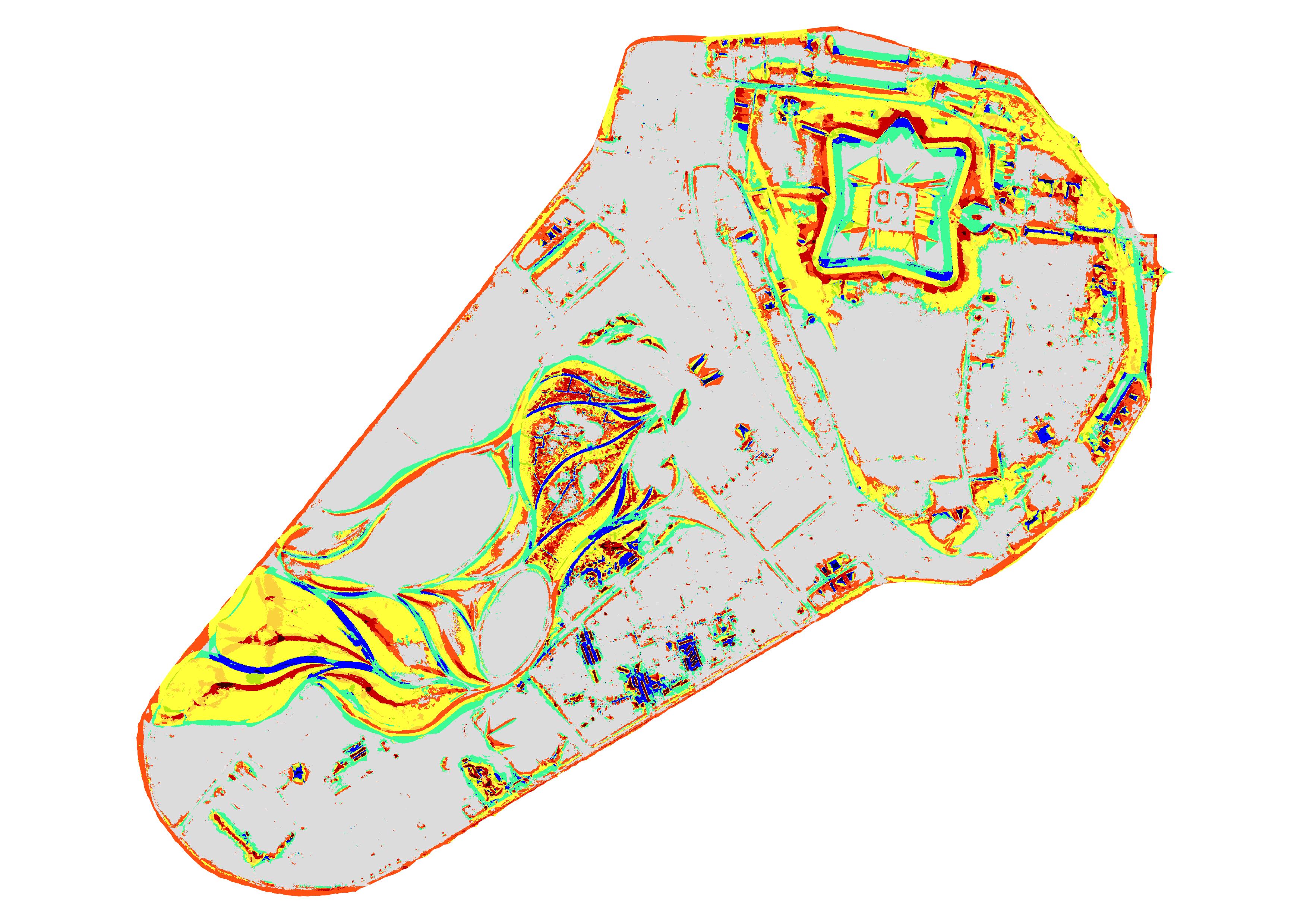 |
To better visualize the landforms,
compute a hillshade using the GRASS module
r.relief.
Under GRASS modules expand raster,
then spatial analysis,
and then terrain analysis.
Double click the module
r.relief
to create a shaded relief map.
In the options tab for r.relief
set the input raster to elevation_2017@PERMANENT,
the output to relief_2017,
and the z-factor to 2 or 3.
Run the module,
click view output to add it to your layer manager and map display,
and then close the module.
Open the layer properties for relief_2017.
In the symbology settings, set the render type to singleband gray and apply.
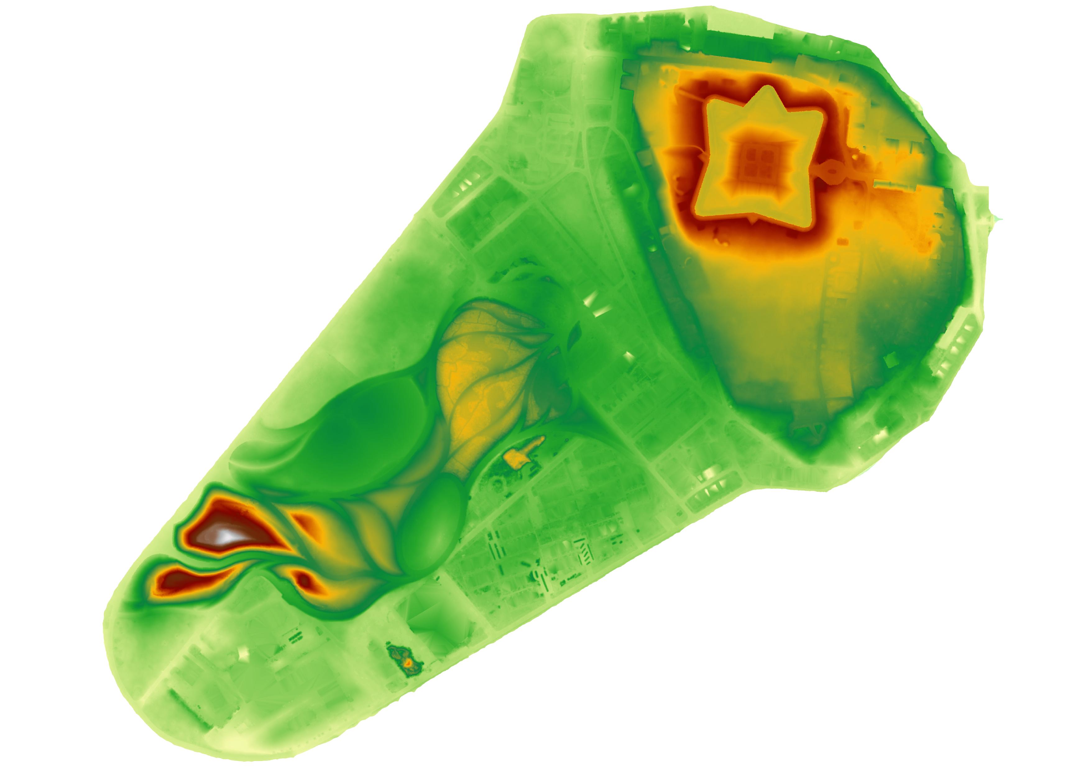
| Shaded Relief |
|---|
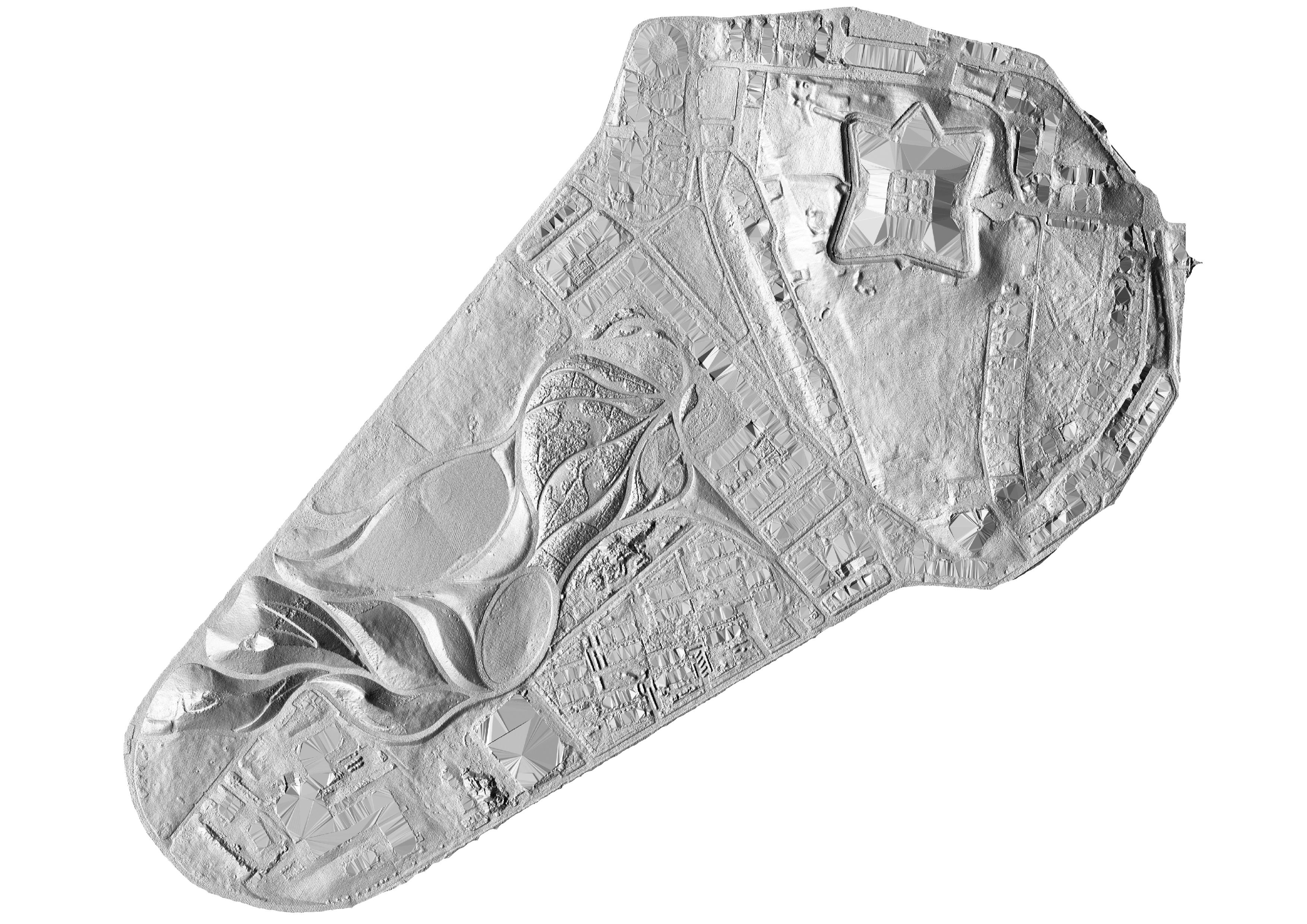 |
To blend the hillshade with the landforms,
open the symbology settings
for relief_2017 again and
set the blending mode to multiply,
brightness to 100, and contrast to 25.
Make sure the layer landforms is turned on and is below layer relief_2017.
| Landforms with Shaded Relief |
|---|
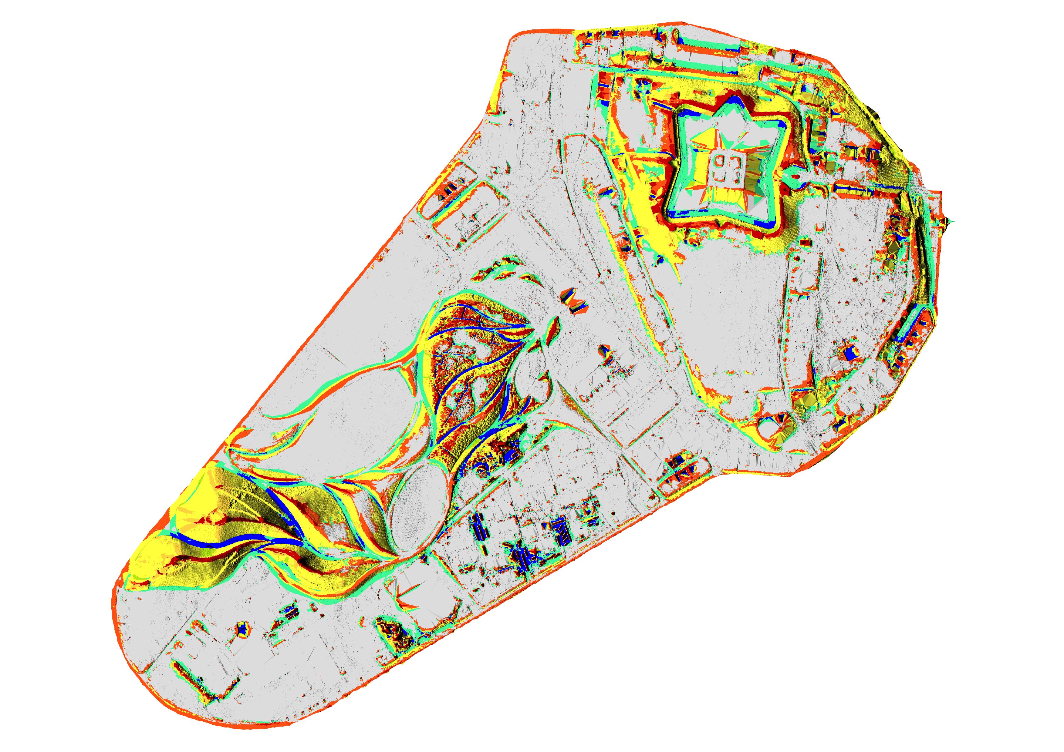 |
To export a high resolution map as an image or a pdf,
go to the Project menu and select New Print Layout.
In the layout window, click add map from the toolbar on the left,
then drag a map window across the canvas snapping on to the corners.
The map of landforms blended with shaded relief will render on the canvas.
Click either the export as image or export as pdf button.
For a high resolution image set the DPI to 300 or greater.
| Print Layout |
|---|
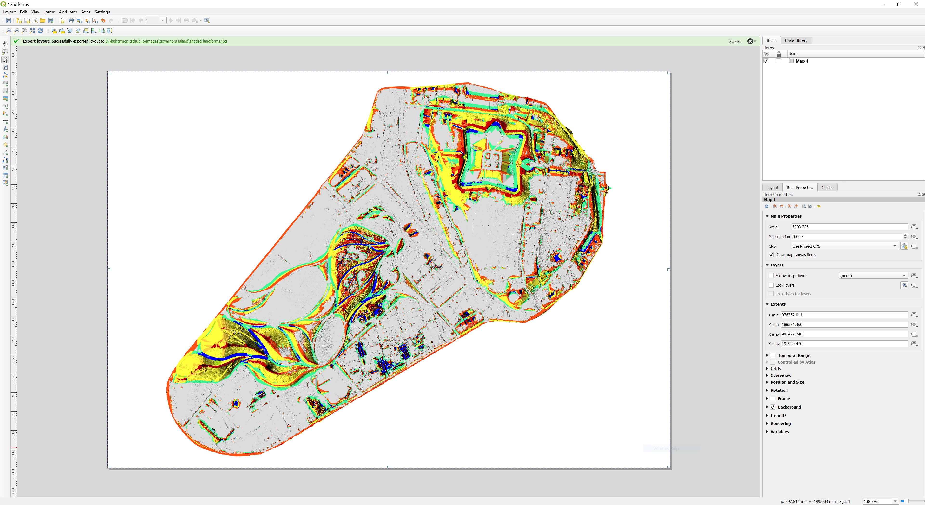 |
GRASS Algorithms
When you want to run GRASS algorithms
with spatial data such as shapefiles, geotiffs, and geopackages
you can use the QGIS Processing Framework.
When you call GRASS algorithms
from the QGIS Processing Framework,
they will not, however, work with GRASS datasets.
This is because they are importing the data into
a GRASS session using r.in.gdal or v.in.ogr.
Download and extract the
Governor’s Island Dataset for QGIS.
Open the project governors_island.qgz
in QGIS Desktop with GRASS.
In the Plugins menu select Manage and Install Plugins.
Check the Processing and GRASS 7 core plugins to enable them.
Check that the layer elevation_2017 appears in the layer manager.
If not, add it from the geopackage governors_island.gpkg.
In the Processing menu, open the Toolbox.
The Processing Toolbox should now be open
in a panel on the right of the screen.
Expand the GRASS section,
expand the Raster section,
and run r.geomorphon to automatically classify landforms.
In the dialog for r.geomorphon,
set the input elevation raster to elevation_2017,
the outer search radius to 36,
the inner search radius to 6,
the flatness threshold to 12,
and the flatness distance to 0.
Under Advanced Parameters
set the region extent to the layer elevation_2017.
Use the default option to save a temporary file.
Run the algorithm.
When the algorithm finishes
it will output a temporary file
for the Most common geomorphic forms.
Open the symbology for the Most common geomorphic forms layer
and export the color map to a file.
Then rename the layer as landforms_2017
and save it to the geopackage governors_island.gpkg.
Open the symbology for landforms_2017,
set the render type to paletted / unique values,
classify, and then load the color map from the saved file.
| Geomorphon Algorithm in the Processing Framework |
|---|
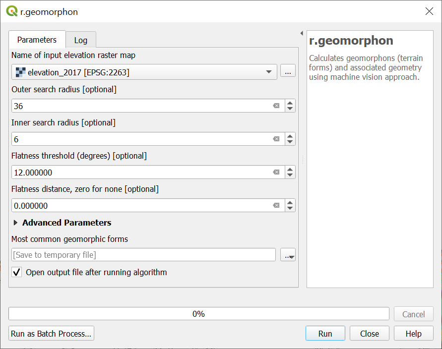 |