Geomorphometry
Quantitative terrain analysis
Contents
Geomorphometry
Geomorphometry is the quantitative analysis of topography. The shape of the earth’s surface – its topographic form – controls processes such as the flow of water and sediment, exposure to sunlight, the distribution of plants, and temperature gradients. At the same time these processes reshape topographic form. Flows of water erode slopes, detaching sediment, then transporting it, and eventually depositing it to build new landforms. The quantitative analysis of form is key to understanding this dynamic relationship between form and process. Topographic form can be visualized based on elevation, illumination, or openness, analyzed in terms of morphometric parameters, and classified by landform type. The free, open source software GRASS GIS GRASS, SAGA, LandLab, WhiteboxTools, and TauDEM have extensive tools for geomorphometric analysis. Geomorphometry can be applied at scales ranging from global (Geomorphons, Geomorpho90, GoogleEarthEngine) to microscopic. This chapter explores site scale applications for Governor’s Island in New York City.
Landscape architects need to understand the shape of the landscape in order to grade the terrain, direct the flow of water, route pathways, and frame views. Landscape architects rely on basic morphometric visualizations such as contours and hillshading to represent topography and draw new designs for landforms. They rely on basic morphometric analyses such as slope and aspect to understand the stability of a hillslope, the walkability of a path, how water will flow across a site, where there will be more sun, and where different plant communities will grow well. Beyond the basic techniques commonly used in the profession, there are many more morphometric visualizations, parameters, and classifications that can reveal much about the shape of the land and its design potential.
While real terrain is made up of discrete rocks, roots, grains of sediment, and so forth, in geomorphometry topography is abstracted as a smooth, continuous surface for the sake of mathematical analysis. Mathematically it is represented as a 2-dimensional manifold in 3-dimensional Euclidean space where elevation \(z\) is a function of the Cartesian coordinates \(x\) and \(y\) (Florinsky 2017):
\[z=f(x,y)\]Continuous surfaces are represented discretely as either raster or mesh grids for numerical analysis. In GRASS topography is represented as a raster grid – a regular array of quadrilateral cells with elevation values (GRASS) – while LandLab can represent topography as a raster grid, hexagonal grid, radial grid, or unstructured, irregular Voronoi-DeLaunay grid (LandLab v2.0). Rasters representing topographic surfaces are called digital elevation models (DEMs). Morphometric parameters can be calculated from digital elevation models using differential calculus.
Box: GIS for Geomorphometry
Figure: Topographic Data Structures
Figure: Geomorpho90
Topographic Visualization
Hypsometry
Contours
Hillshade
Skyview
Principle Components
Morphometric Parameters
Morphometric parameters – such as slope, aspect, and curvature – can be derived from a topographic surface. These parameters quantitatively describe the morphology of the terrain. In GRASS the basic morphometric parameters – slope, aspect, and curvature – can be approximated from a raster digital elevation model using polynomials with the module r.slope.aspect (Geomorphometry in GRASS) or r.param.scale (Wood) or computed from a point cloud using spline interpolation with the module v.surf.rst (Mitasova). Other morphometric parameters such as the Laplacian can be computed from partial derivatives using map algebra. This chapter covers methods using approximation from polynomials, while Chapter 5 covers spline interpolation.
Box: Morphometric Parameters
Figure: Grid of morphometric parameters
Volume
The volume of the topographic surface \(z=f(x,y)\) can be approximated as the sum of cuboids, i.e. of raster grid cells’ area multiplied by their elevation above a datum. By representing a surface as a raster with regular grid cells, the volume of each cell can be computed by multiplying its resolution in the x-axis by its resolution in the y-axis by its elevation above a datum.
\[V = \sum dx \cdot dy \cdot dz\]where:
\(V\) is volume
\(dx\) is east-west resolution
\(dy\) is north-south resolution
\(dz\) is elevation
The datum may be a constant value such as sea level or another surface from for example a cut and fill operation. In GRASS volume can be computed either using map algebra and univariate statistics with r.mapcalc and r.univar or using the module r.volume.
GRASS CLI
r.volume input=elevation
Elevation Gradient
The elevation gradient \(\nabla z\) is the vector field representing the maximum rate of change in elevation for the topographic surface \(z=f(x,y)\). Vectors represent magnitude and direction so the vector field of a topographic surface represents the magnitude and direction of change in elevation for each point on the surface. Vector fields can be represented as a set of points with arrows pointing in the direction of change and scaled by the magnitude of change. Mathematically the elevation gradient \(\nabla z\) can be represented by the maximum rate of change in the x direction and the maximum rate of change in the y direction, i.e. the first order partial derivatives \(\frac{\partial z}{\partial x}\) and \(\frac{\partial z}{\partial x}\).
\[\nabla z = \left( \frac{\partial z}{\partial x}, \frac{\partial z}{\partial y} \right)\]where:
\(\nabla z\) is the gradient vector
\(\frac{\partial z}{\partial x}\) is the first order partial derivative in the x direction
\(\frac{\partial z}{\partial y}\) is the first order partial derivative in the y direction
Figure Vector as magnitude and direction between points A and B. Show Grasshopper diagram.
Figure Elevation gradient for the Governor’s Island landforms from Docofossor.
Partial Derivatives
The first order partial derivatives of elevation \(\frac{\partial z}{\partial x}\) and \(\frac{\partial z}{\partial y}\) represent the maximum rate of change in elevation in the x and y directions. The partial derivatives of a topographic surface can be estimated using polynomial approximation with Horn’s formula (Horn, 1981; Neteler and Mitášová, 2008). When the continuous surface \(z=f(x,y)\) is discretized as a raster, the partial derivatives for each grid cell can be estimated using polynomial approximation over the 3 x 3 neighborhood of cells centered on the cell (Geomorphometry in GRASS, p.397). The first order partial derivatives \(\frac{\partial z}{\partial x}\) and \(\frac{\partial z}{\partial y}\) are used to calculate slope and aspect, while the first and second order partial derivatives \(\frac{\partial z^2}{\partial x^2}\), \(\frac{\partial z^2}{\partial y^2}\), and \(\frac{\partial z^2}{\partial xy}\) are used to calculate curvature and the divergence of the elevation gradient.
Figure: 3 x 3 Neighborhood
First order partial derivatives
\[\frac{\partial z}{\partial x} = \frac{(z_7-z_9)+(2z_4-2z_6)+(z_1-z_3)}{8 \Delta x}\] \[\frac{\partial z}{\partial y} = \frac{(z_7-z_1)+(2z_8-2z_2)+(z_9-z_3)}{8 \Delta y}\]Second order partial derivatives
\[\frac{\partial z^2}{\partial x^2} = \frac{z_1 - 2z_2 + z_3 + 4z_4 + 8z_5 + 4z_6 + z_7 - 2z_8 + z_9}{6 \Delta x^2}\] \[\frac{\partial z^2}{\partial y^2} = \frac{z_1 + 2z_2 + z_3 - 2z_4 - 8z_5 - 2z_6 + z_7 + 4z_8 + z_9}{6 \Delta y^2}\] \[\frac{\partial z^2}{\partial xy} = \frac{(z_7-z_9)-(z_1-z_3)}{4 \Delta x \Delta y}\]In GRASS partial derivatives and other basic morphometric parameters can be calculated from a digital elevation model with the module r.slope.aspect.
GRASS CLI
r.slope.aspect -e elevation=elevation dx=dx dy=dy dxx=dxx dyy=dyy dxy=dxy
GRASS Python
gscript.run_command(
    'r.slope.aspect',
    elevation='elevation',
    dx='dx',
    dy='dy',
    dxx='dxx',
    dyy='dyy',
    dxy='dxy',
    overwrite=True)
Slope
Slope \(\gamma\) is the magnitude of the elevation gradient \(\nabla z\). It is a measure of steepness and can be represented in degrees, as a percentage, or as a ratio. Slope can also be classified by categories for simpler visualization and easier decision making. It is a key parameter for landscape architects because it determines the stability and walkability of the terrain and the velocity of overland flows of water and sediment. Slope is the vertical change in elevation over the horizontal change in distance \(\frac{dz}{dxy}\), i.e. rise over run. The slope of a surface can be calculated by combining the partial derivatives \(\frac{\partial z}{\partial x}\) and \(\frac{\partial z}{\partial y}\) (Wood, p.84-85, Florinsky 2017).
Slope \(\gamma\) is the magnitude of the elevation gradient \(\nabla z\). It is a measure of steepness and can be represented in degrees, as a percentage, or as a ratio. It is a key parameter for landscape architects because it determines the stability and walkability of the terrain and the velocity of overland flows of water.
\[\frac{dz}{dxy} = \sqrt{ \left( \frac{\partial z}{\partial x} \right)^2 + \left( \frac{\partial z}{\partial y} \right)^2}\]where:
\(\frac{dz}{dxy}\) is slope
\[\gamma = \arctan \sqrt{ \left( \frac{\partial z}{\partial x} \right)^2 + \left( \frac{\partial z}{\partial y} \right)^2}\]where:
\(\gamma\) is slope angle
\[\gamma \% = 100 \cdot \sqrt{ \left( \frac{\partial z}{\partial x} \right)^2 + \left( \frac{\partial z}{\partial y} \right)^2}\]where:
\(\gamma \%\) is slope magnitude
In GRASS
slope can be computed using either
r.param.scale
or
r.slope.aspect.
Both modules use a moving window
for polynomial approximation over a neighborhood of cells.
While r.slope.aspect
uses a 3 x 3 neighborhood,
the width of the neighborhood used by
r.param.scale
is set with the size parameter
so that slope can be calculated at different scales.
High resolution digital elevation models
derived from lidar or drone photogrammetry
may have so much detail that geomorphometric analyses
appear too noisy to be legible.
Using a larger moving window effectively smooths the elevation data
resulting in a simpler, more legible pattern of slope.
To compute slope at different scales with
r.slope.aspect
first smooth the digital elevation model using
r.neighbors.
The module r.neighbors
conducts a statistical analysis of the neighborhood surrounding each cell
using a moving window of given size.
Setting its method to average will smooth data
such as a digital elevation model.
GRASS CLI
r.param.scale input=elevation output=slope method=slope size=3
GRASS Python
gscript.run_command(
    'r.param.scale',
    input='elevation',
    output='slope',
    method='slope',
    size=3)
GRASS CLI
r.slope.aspect -e elevation=elevation slope=slope format=degrees
GRASS Python
gscript.run_command(
    'r.slope.aspect',
    elevation='elevation',
    slope='slope',
    format='degrees')
Aspect
Aspect \(\alpha\) is the direction of the elevation gradient \(\nabla z\). It ranges from 0 to 360 degrees. Aspect represents flow direction, the direction that water and sediment will flow under the force of gravity. It can also be used for hillshading and determining solar orientation. Aspect is an important geomorphometric parameter for landscape architects as flow direction governs drainage and solar orientation is a factor in where plants will grow. Like slope, aspect can be calculated from the first order partial derivatives of the topographic surface.
\[\alpha = \arctan \frac{ \left( \frac{\partial z}{\partial x} \right) }{ \left( \frac{\partial z}{\partial y} \right) }\]In GRASS aspect can be computed with either the module r.param.scale or r.slope.aspect.
GRASS CLI
r.param.scale input=elevation output=aspect method=aspect size=3
GRASS Python
gscript.run_command(
    'r.param.scale',
    input='elevation',
    output='aspect',
    method='aspect',
    size=3)
GRASS CLI
r.slope.aspect -e elevation=elevation aspect=aspect
GRASS Python
gscript.run_command(
    'r.slope.aspect',
    elevation='elevation',
    aspect='aspect',
    overwrite=True)
Curvature
Curvature is the deviation of a surface from a reference plane in \(m^{-1}\). It varies by direction. For landscape architects curvature is useful for analyzing flows and identifying landforms. There are many types of curvature including minimum, maximum, mean, Gaussian, plan, profile, tangential, difference, accumulation, and others (Wood 1996, Florinsky 2017). Of these profile and tangential curvature are among the most useful for geomorphometric analysis.
Profile curvature \(K_p\) is the curvature in the direction of the elevation gradient \(\nabla z\). It is a measure of the rate of change in slope and the acceleration of flows. When profile curvature is concave, the slope is decreasing and flows are decelerating. Conversely, when it is convex, the slope is increasing and flows are accelerating. Tangential curvature \(K_t\) is the curvature perpendicular to the elevation gradient \(\nabla z\), i.e. tangent to the contour. It is a measure of the convergence of flows. Both profile and tangential curvature can be calculated from first and second order partial derivatives of the topographic surface \(z=f(x,y)\).
\[K_p = \frac{ \left( \frac{\partial^2 z}{\partial x^2} \right) \left( \frac{\partial z}{\partial x} \right)^2 + 2 \left( \frac{\partial^2 z}{\partial x \partial y} \right) \left( \frac{\partial z}{\partial x} \right) \left( \frac{\partial z}{\partial y} \right) + \left( \frac{\partial^2 z}{\partial y^2} \right) \left( \frac{\partial z}{\partial y} \right)^2 }{ \left( \frac{\partial z}{\partial x} \right)^2 + \left( \frac{\partial z}{\partial y} \right)^2 \sqrt{\left( 1 + \left( \frac{\partial z}{\partial x} \right)^2 + \left( \frac{\partial z}{\partial y} \right)^2 \right)^3 } }\]where:
\(K_p\) is profile curvature
\[K_t = \frac{ \left( \frac{\partial^2 z}{\partial x^2} \right) \left( \frac{\partial z}{\partial y} \right)^2 - 2 \left( \frac{\partial^2 z}{\partial x \partial y} \right) \left( \frac{\partial z}{\partial x} \right) \left( \frac{\partial z}{\partial y} \right) + \left( \frac{\partial^2 z}{\partial y^2} \right) \left( \frac{\partial z}{\partial x} \right)^2 }{ \left( \frac{\partial z}{\partial x} \right)^2 + \left( \frac{\partial z}{\partial y} \right)^2 \sqrt{ 1 + \left( \frac{\partial z}{\partial x} \right)^2 + \left( \frac{\partial z}{\partial y} \right)^2 } }\]where:
\(K_t\) is tangential curvature
In GRASS curvature can be computed with either r.param.scale or r.slope.aspect. % While r.slope.aspect can compute profile and tangential curvature, r.param.scale can compute profile, plan, longitudinal, cross-sectional (i.e. tangential), minimum, and maximum curvature.
GRASS CLI
r.param.scale input=elevation output=profc method=profc size=3
r.param.scale input=elevation output=crosc method=crosc size=3
GRASS Python
gscript.run_command(
    'r.param.scale',
    input='elevation',
    output='profc',
    method='profc',
    size=3)
gscript.run_command(
    'r.param.scale',
    input='elevation',
    output='crosc',
    method='crosc',
    size=3)
GRASS CLI
r.slope.aspect -e elevation=elevation pcurvature=pcurvature tcurvature=tcurvature
GRASS Python
gscript.run_command(
    'r.slope.aspect',
    elevation='elevation',
    pcurvature='pcurvature',
    tcurvature='tcurvature')
Laplacian
For the topographic surface \(z=f(x,y)\) the Laplacian \(\nabla ^2\) is the divergence of the elevation gradient in \(m^{-1}\) (Laplace 1799, Florinsky 2017). As a morphometric parameter, it can be used to calculate the gravitational diffusion of sediment and classify convergent or divergent landforms. The Laplacian can be calculated as the sum of the second order partial derivatives \(\frac{\partial^2 z}{\partial x^2}\) and \(\frac{\partial^2 z}{\partial y^2}\):
\[\nabla ^2 = \frac{\partial^2 z}{\partial x^2} + \frac{\partial^2 z}{\partial y^2}\]In GRASS the Laplacian can be computed by calculating the second order partial derivatives \(\frac{\partial^2 z}{\partial x^2}\) and \(\frac{\partial^2 z}{\partial y^2}\) of digital elevation model with the module r.slope.aspect and then adding them together using map algebra with the module r.mapcalc.
GRASS CLI
r.slope.aspect elevation=elevation dxx=dxx dyy=dyy
r.mapcalc expression="laplacian = dxx + dyy"
GRASS Python
gscript.run_command(
    'r.slope.aspect',
    elevation='elevation',
    dxx='dxx',
    dyy='dyy',
    overwrite=True)
gscript.mapcalc("laplacian = dxx + dyy")
Local Relief
Topographic Index
Stream Power Index
Landform Classification
Concavity and Convexity
Divergence and Convergence
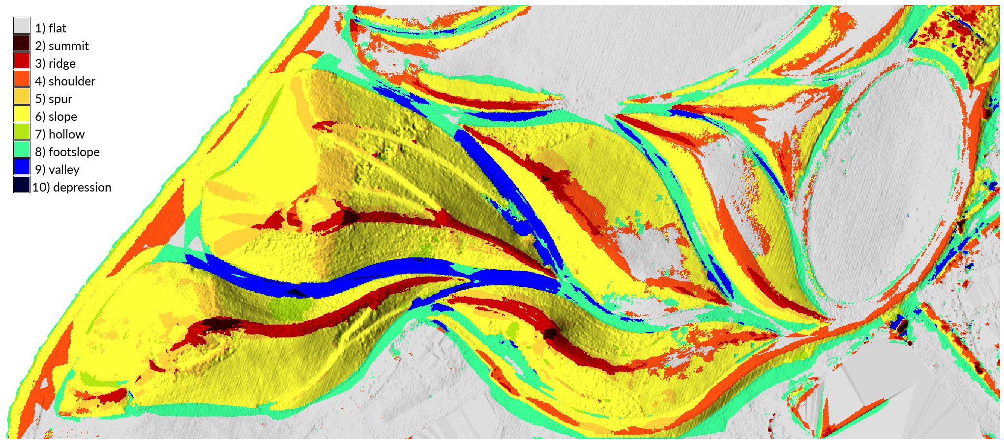
Geomorphons
Exercises
Cut-fill Volume
Compute the change in volume from 2014 to 2017 for the Governor’s Island landforms
- using command line
- using Python
Morphometric Parameters
- using command line
- using Python