Contents

• Census Data
• Download Census Data
• Importing Census Data
• Choropleth Maps
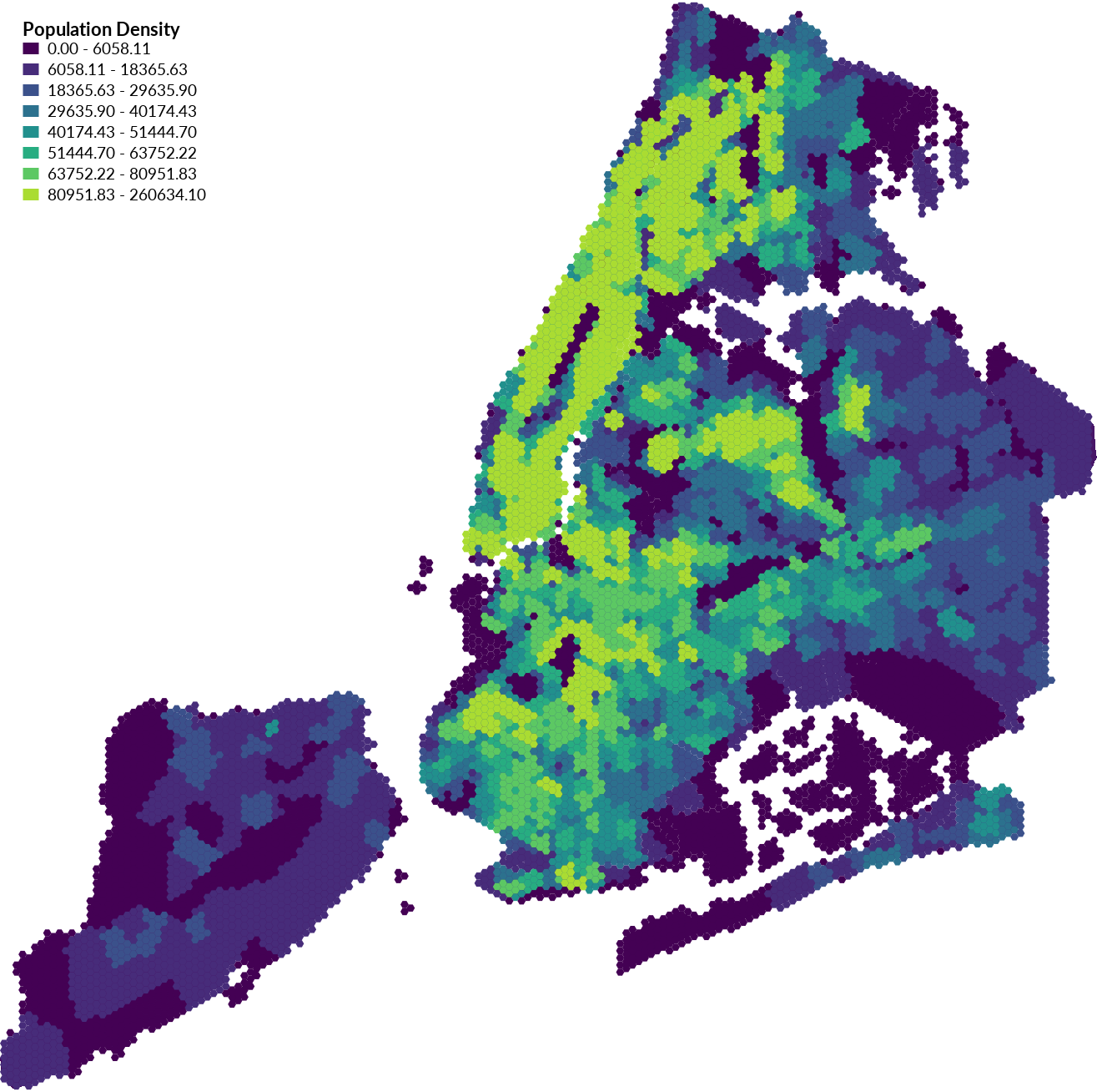
• Hexagonal Binning Map
• Resources

Census Data

This tutorial is an introduction to mapping demographic data in GRASS GIS. Every 10 years the US Census Bureau conducts a census collecting demographic information from US residents and publishes aggregated statistics. In addition to the decennial census, the US Census Bureau also conducts the American Community Survey (ACS) collecting more detailed information from a sample of the population every month. To protect people’s privacy only aggregated statistical data is published. Census data is aggregated for geographic regions at scales ranging from the nation to states to counties to tracts to block groups to blocks. Use data from the American Community Survey to map the estimated population density of each census tract in New York City.

Download Census Data

To find and download tabular data from the US Census Bureau go to data.census.gov. Search for the survey ACS Demographic and Housing Estimates or table DP05. Select the table DP05. Select the product 2018: ACS 5-Year Estimates Data Profiles. Only the 5-year estimates have census tract and block group level data. Click customize table. Set Geos to select a geographic region and level of detail. Select Tract, within New York state, all census tracts within New York Then Download the table as a csv for 2018.

Survey: ACS DEMOGRAPHIC AND HOUSING ESTIMATES
Survey: ACS
Table ID: DP05
Product: 2018: ACS 5-Year Estimates Data Profiles
Geo:
Geography: Tract
Tract: New York
Within: all census tracts within New York
Download as csv

Edit the .csv table in a spreadsheet program such as Excel or LibreOffice Calc. Delete the second row that describes each column, then use find and replace to remove the prefix 1400000US from the first column with GEO_IDs. Since deleting all unneeded columns will dramatically improve performance, delete all columns except for GEO_ID, NAME, and DP05_0033E with total population estimates. Save the table as population.csv.

To be mapped the tabular demographic data from the census needs to be joined to geospatial data for the appropriate geographic regions, in this case the census tracts for New York. The Topologically Integrated Geographic Encoding and Referencing (Tiger/Line) database contains spatial data for roads, rail, buildings, hydrography, and geographic regions in the US including census tracts and block groups. Find and download the TIGER/Line shapefile for the census tracts in New York at https://www.census.gov/cgi-bin/geo/shapefiles/index.php. Set the year to 2018, layer type to census tracts, and state to New York. Download and extract tl_2018_36_tract.zip. The tables with demographic data and the census tract shapefiles share geographic entity codes (GEOIDs) that can be used to join them. Also download and extract borough boundaries for New York City from NYC Open Data. The borough boundaries will be used to specify the study area for mapping.

Importing Census Data

For this tutorial either create a new location in New York Long Island State Plane Feet or use the Governor’s Island Dataset for GRASS GIS. To create a new location for New York Long Island State Plane Feet start GRASS GIS and create a new location based on EPSG code 2263 or the georeferenced file nybb.shp from the borough boundaries. Alternatively download, extract, and move the Governor’s Island Dataset for GRASS GIS to your grassdata directory. Start GRASS GIS, set the GRASS GIS database directory to grassdata directory, set the location to nyspf_govenors_island, and create a new mapset called census.

First import the borough boundaries with v.in.ogr. Then import and reproject the census tract boundaries for the state of New York with v.import. Clip the census tract boundaries to the boroughs with v.clip. Import population.csv as a table with db.in.ogr and then join this table to the census tracts’ attribute table with v.db.join. Set the identifier column to GEOID from the census tract attribute table and the other column to GEO_ID from the population table. For this to work the prefix 1400000US must have been stripped from all entries in the GEO_ID column. Joining may take a very long time if all unnecessary rows and columns were not deleted from population.csv. The column DP05_0033E with population data will be interpreted as a text column with the TEXT string data type. To map the population data, create a new column with the data type set to INT for integer using v.db.addcolumn and then copy the population values from the text column to the new numeric column with v.db.update. For v.db.update use the query DP05_0033E >= 0 to only copy values greater than or equal to zero. Set the color table for the vector map of census tracts to the numeric population column in the attribute table with v.colors.

v.import input=tl_2018_36_tract.shp layer=tl_2018_36_tract output=nyc_census_tracts
v.in.ogr input=nybb.shp output=boroughs
v.clip input=nyc_census_tracts clip=boroughs output=census_tracts
db.in.ogr input=population.csv output=population
v.db.join map=census_tracts column=GEOID other_table=population other_column=GEO_ID
v.db.addcolumn map=census_tracts columns="population INT"
v.db.update map=census_tracts column=population query_column=DP05_0033E where="DP05_0033E >= 0"
v.colors map=census_tracts use=attr column=population color=viridis

To compute population density per census tract first use v.db.addcolumn to create a new column called density with the data type set to REAL for floating point values, i.e. numbers with decimal places. Then use v.db.update to compute population density per square mile and populate the new density column. Since the column ALAND from the census tracts has the area per square meter divide it by 2,589,988 to convert it to area per square mile and then divide the population column by converted area.

v.db.addcolumn map=census_tracts columns="density REAL"
v.db.update map=census_tracts column=den query_column=population/(ALAND/2589988.0)

Choropleth Maps

Choropleth maps color or pattern geographic areas in proportion to an aggregated variable. Use d.vect.thematic to create a choropleth map of the population density of New York City by census tract. Set the input map to the vector map of census tracts, the attribute column to the numeric population column, the algorithm to a normal distribution with equ, the number of classes to 9, and the color table to viridis with 9 classes with following rules:

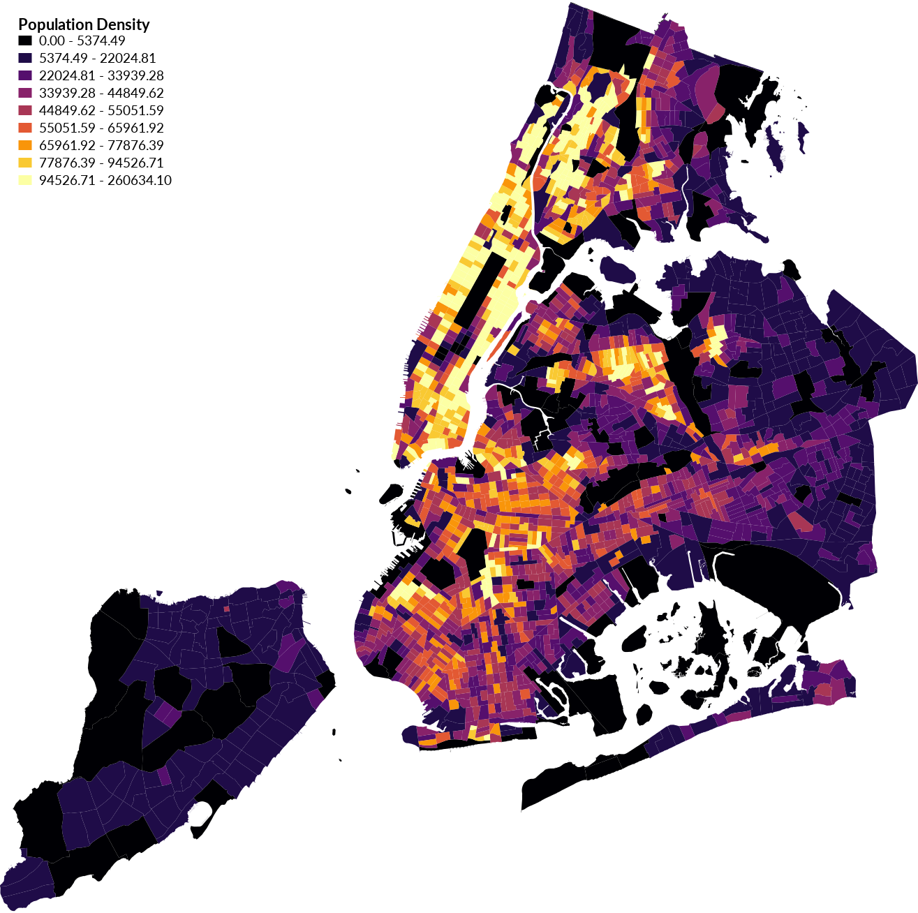
68:1:84,71:44:122,59:81:139,44:113:142,33:144:141,39:173:129,92:200:99,170:220:50,253:231:37

Add a vector legend with d.legend.vect. Optionally use d.vect.chart to plot bar charts of the population density per census tract.

d.vect.thematic -l --overwrite map=census_tracts column=density algorithm=equ nclasses=9 colors=68:1:84,71:44:122,59:81:139,44:113:142,33:144:141,39:173:129,92:200:99,170:220:50,253:231:37 boundary_color=none legend_title="Population Density"
d.legend.vect at=2,98 font=Lato-Regular fontsize=14 sub_font=Lato-Bold sub_fontsize=16
d.vect.chart -3 map=census_tracts chart_type=bar columns=density size_column=1 size=1 scale=0.0003

Population Density Choropleth

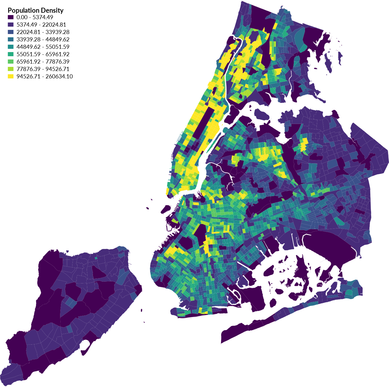Experiment with different algorithms, numbers of classes, and color rules. For example try setting the algorithm to quantile instead of normal distribution with algorithm=qua. To set the color table to inferno with 9 classes use the following rules:

0:0:4,31:12:72,85:15:109,136:34:106,168:54:85,227:89:51,249:149:10,249:201:50,252:255:164

Population Density Quantiles Choropleth

To easily generate color rules visit ColorBrewer. For example pick the second sequential, multi-hued color scheme with 9 classes and RGB output to generate the following rules:

247:252:253,224:236:244,191:211:230,158:188:218,140:150:198,140:107:177,136:65:157,129:15:124,77:0:75

Population Density Choropleth with Sequential Colors

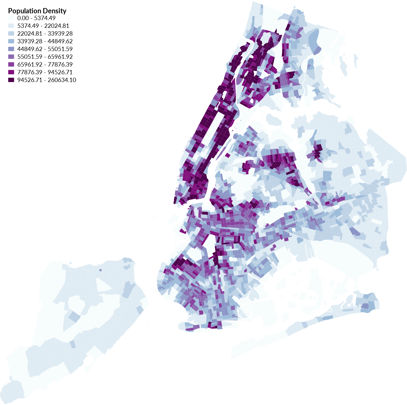Use the addon module m.printws to print the workspace as a high resolution PDF. First export the vector legend as legend.csv with d.legend.vect and then import it so that the legend will save as part of the workspace. Save the workspace as population_density.gxw navigate through the file menu to workspace and select then save as. After saving the workspace run m.printws with the input set to population_density.gxw, dots per inch (dpi) set to 300, and page size set to fit the data with Flexi.

d.legend.vect at=1,98 font=Lato-Light fontsize=48 sub_font=Lato-Medium output=legend.csv --overwrite
d.legend.vect at=1,98 font=Lato-Light fontsize=48 sub_font=Lato-Medium input=legend.csv --overwrite
m.printws --overwrite input=population_density.gxw dpi=300 output=population_density page=Flexi

High resolution population density choropleth

Hexagonal Binning Map

Resample the population density data to create a hexagonal binning (hexbin) map. First set the computational region to the vector map of census tracts with g.region. Then rasterize the population density from the vector map of census tracts with v.to.rast by setting the attribute column to density. Then create a hexagonal grid with v.mkgrid based on the current region. Set the -h flag to generate a hexagonal grid and set the size of each hexagon with the box parameter. Experiment with different sized hexagons. Use v.select to select only hexagons that intersect with boroughs. Set the first input to the hexagonal grid, the second input to boroughs, and the operator to intersects. Then calculate univariate statistics for each hexagon from the raster map of population density with v.rast.stats. Use d.vect.thematic to create a hexbin map of the population density. Set the attribute column to average or maximum density. Then add a vector legend with d.legend.vect.

g.region vector=census_tracts res=100
v.to.rast input=census_tracts output=density use=attr attribute_column=density
v.mkgrid -h map=grid box=1000,1000
v.select ainput=grid binput=boroughs output=hexagons operator=intersects
v.rast.stats -c map=hexagons raster=density column_prefix=density
d.vect.thematic -l --overwrite map=hexagons column=density_maximum algorithm=equ nclasses=9 colors=68:1:84,71:44:122,59:81:139,44:113:142,33:144:141,39:173:129,92:200:99,170:220:50,253:231:37 boundary_color=none legend_title="Population Density"
d.legend.vect at=2,98 font=Lato-Regular fontsize=14 sub_font=Lato-Bold sub_fontsize=16

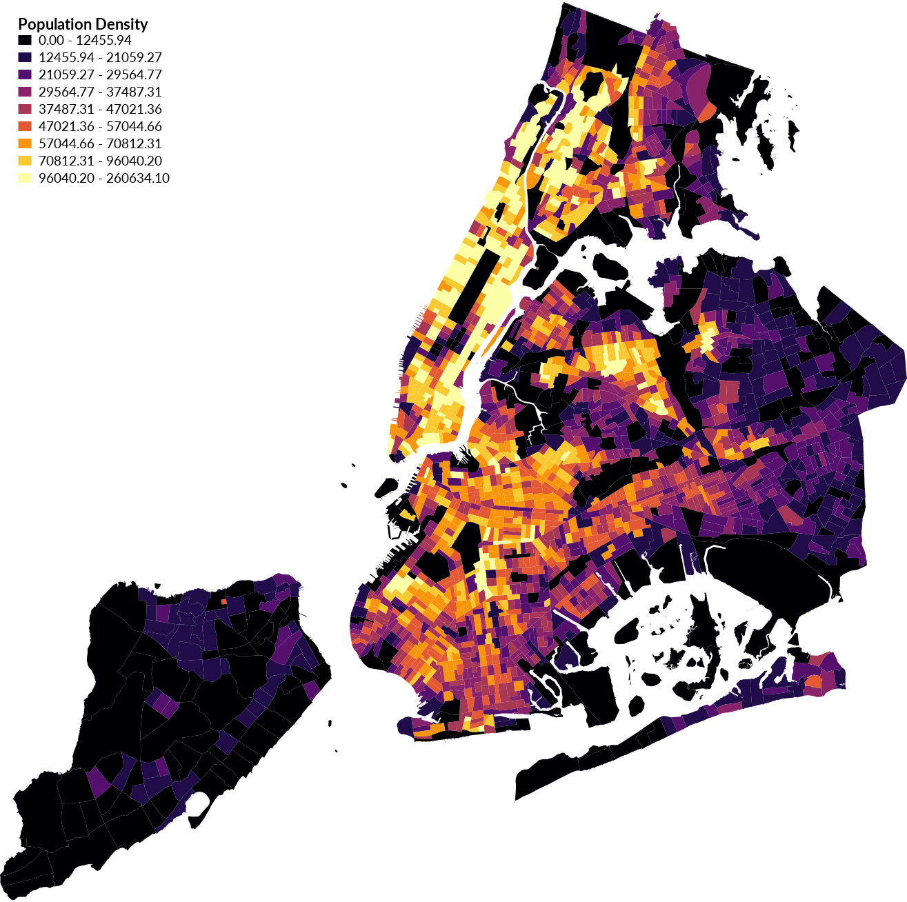
Hexagonal Binning of Population Density

Save and then print the workspace as a high resolution PDF with m.printws.

d.legend.vect at=1,98 font=Lato-Light fontsize=48 sub_font=Lato-Medium output=D:\grassdata\nyspf_govenors_island\hexbin_legend.csv --overwrite
d.legend.vect at=1,98 font=Lato-Light fontsize=48 sub_font=Lato-Medium input=D:\grassdata\nyspf_govenors_island\hexbin_legend.csv --overwrite
m.printws --overwrite input=D:\grassdata\nyspf_govenors_island\hexbin.gxw dpi=300 output=D:\grassdata\nyspf_govenors_island\population_density_hexbin page=Flexi

Hexagonal Binning of Population

Resources

For a discussion of choropleth maps and an in depth guide to mapping in R read the maps chapter of Kieran Healy’s book Data Visualization: A practical introduction.