Contents

• Dataset
• Computational Region
• Hillshade
• Skyview Factor
• Contours
• Slope

Dataset

Download and extract the Governor’s Island Dataset for GRASS GIS. This geospatial dataset contains raster and vector data for Governor’s Island, New York City, USA. The top level directory nyspf_governors_island is a GRASS GIS location for  NAD 1983 State Plane New York Long Island FIPS 3104 Feet in US Surveyor’s Feet. Inside the location there is the PERMANENT mapset, a license file, data record, readme file, workspace, color table, category rules, and scripts for data processing. Data sources include http://gis.ny.gov/, https://orthos.dhses.ny.gov/ and https://data.cityofnewyork.us/. Create a directory on your computer called grassdata. This will be your GRASS GIS database directory where you will store your GRASS locations and mapsets. Move the location nyspf_govenors_island inside of your grassdata directory.

Computational Region

Start GRASS GIS, set the GRASS GIS database directory to the directory grassdata, select nyspf_governors_island as your location, and create a new mapset called terrain_analysis. While we will have access to reference data in the PERMANENT mapset, all new data will be created in the new terrain_analysis mapset. Set your computational region to cover the landforms in the southwest of the island. Zoom in and use the various zoom options dialog in the graphical user interface (GUI) to Set computational region from display. Alternatively run g.region and set the boundaries listed below for the region. Save your custom region using the various zoom options dialog Save computational region as named region. Then set a mask to the vector map shoreline with the module r.mask.

g.region n=189850 s=189100 e=978550 w=976850 res=1 save=landforms
r.mask vector=shoreline

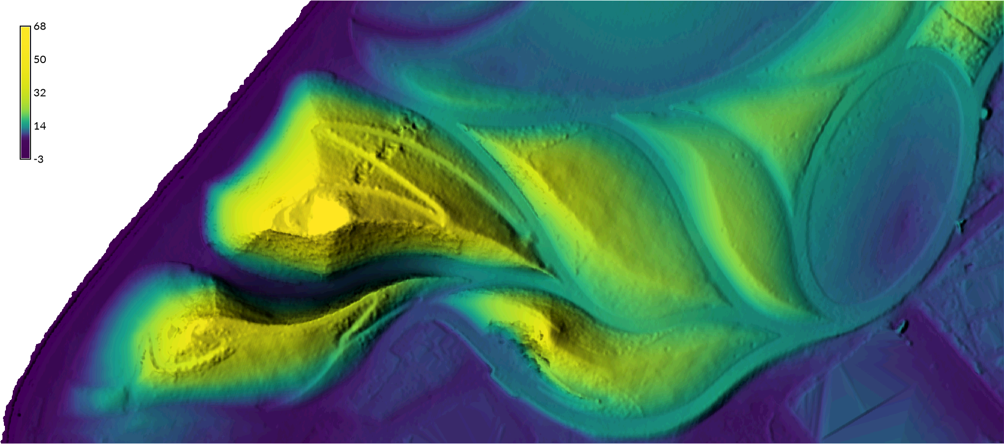
Digital Elevation Model

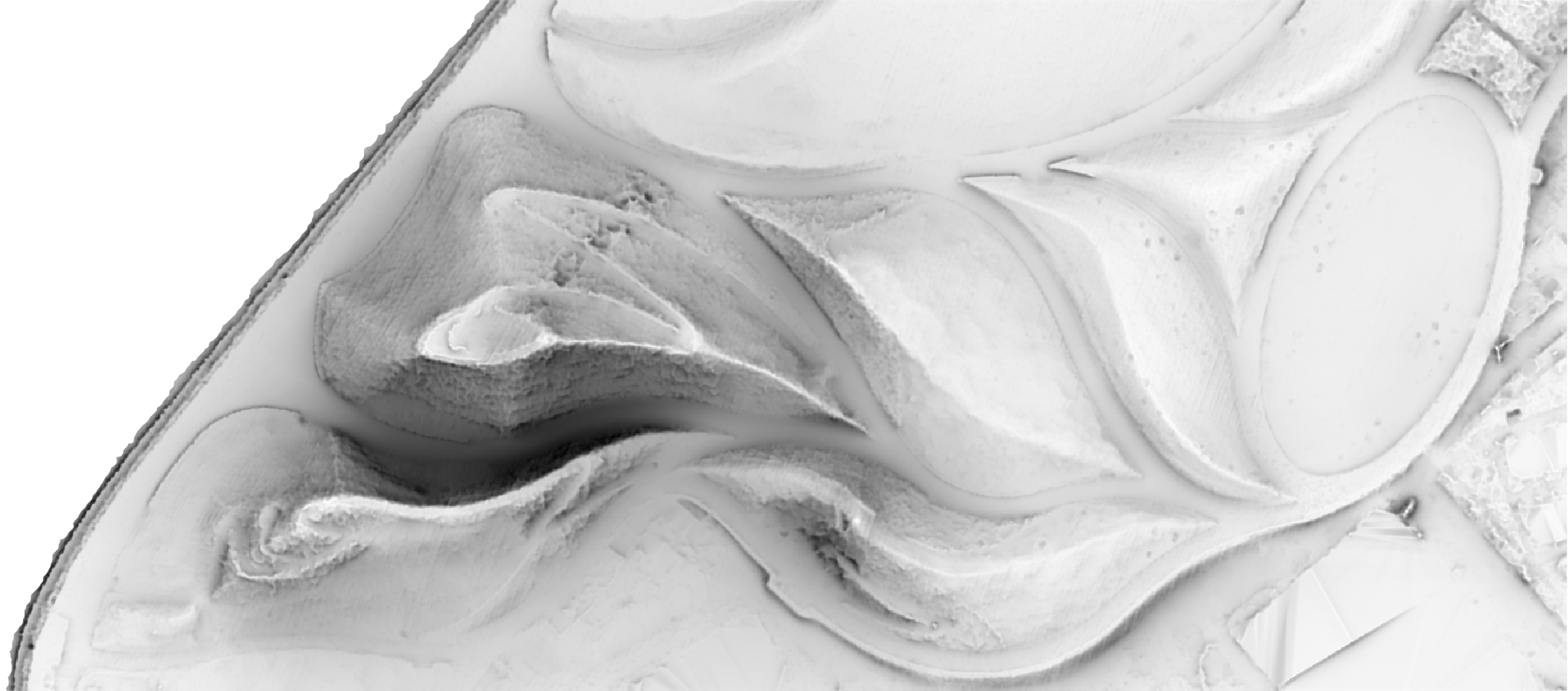
Hillshade

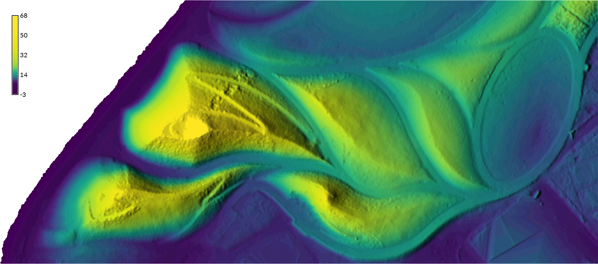
Visualize the relief of the terrain using direct illumination with r.relief. Set elevation to the map elevation_2017 in the PERMANENT mapset and set the units parameter to survey feet. The light source can be set using the altitude and azimuth parameters.

r.relief input=elevation_2017 output=relief zscale=2 units=survey

Shaded Relief

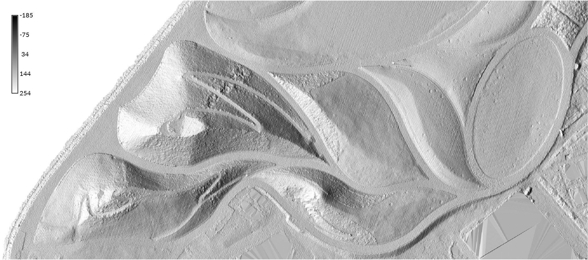Noise from the lidar data shows up clearly in the relief map. Note the parallel lines running diagonally across the landscape - these are noise from the lidar data. To reduce noise smooth the digital elevation model using the module r.neighbors with a circular neighborhood with a 5 ft diameter. This will create a new smoothed elevation map cropped to the region in the current mapset, while leaving the original elevation map unchanged in the PERMANENT mapset. 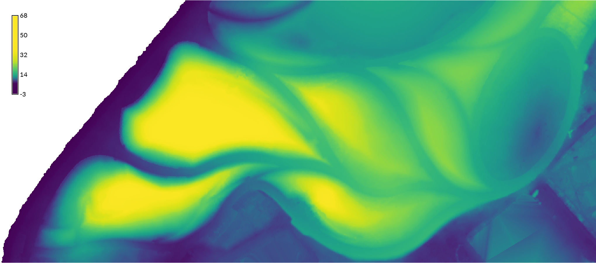Use r.colors to set the color table for the cropped and smoothed elevation map to viridis or elevation with the flag -e for histogram equalization. 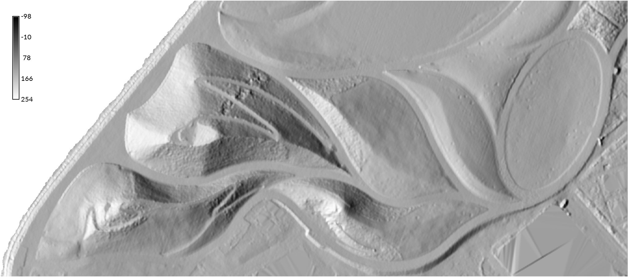Now compute hillshading for the smoothed digital elevation model with the module r.relief. Set the --overwrite flag to replace the relief map. Then overlay the elevation map over the hillshade using the module r.shade. Set the brighten parameter to 36. Add a legend with d.legend.

r.neighbors -c input=elevation_2017 output=elevation size=7
r.colors -e map=elevation color=viridis
r.relief --overwrite input=elevation output=relief zscale=2 units=survey
r.shade shade=relief color=elevation output=shaded_relief brighten=36
d.legend raster=elevation at=70,96,2,3 font=Lato-Regular fontsize=14

Smoothed Shaded Relief

Digital Elevation Model with Shaded Relief

Skyview Factor

Try visualizing relief using diffuse illumination from the skyview factor - the proportion of the sky visible given the surrounding relief. First install the addon module r.skyview with g.extension. Then compute the skyview factor with r.skyview from 16 directions. A composite of the shaded relief and skyview factor will combine direct and diffuse illumination to better visualize relief. Use r.shade to drape the shaded relief map over the skyview factor.

g.extension extension=r.skyview
r.skyview input=elevation output=skyview ndir=16
r.shade shade=skyview color=shaded_relief output=composite_relief brighten=80
d.legend raster=elevation at=60,95,2,3.5 font=Lato-Regular fontsize=14

Skyview Factor

Digital Elevation Model with Direct and Diffuse Illumination

Contours

Compute contours at 3 ft intervals from the smoothed digital elevation model using the module r.contour. To further reduce noise, use the cut parameter to specify the minimum number of points per contour curve.

r.contour input=elevation output=contours_3ft step=3 cut=100

3 ft Contours

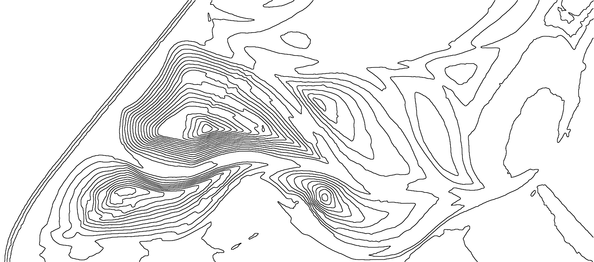Skyview Factor with 3 ft Contours

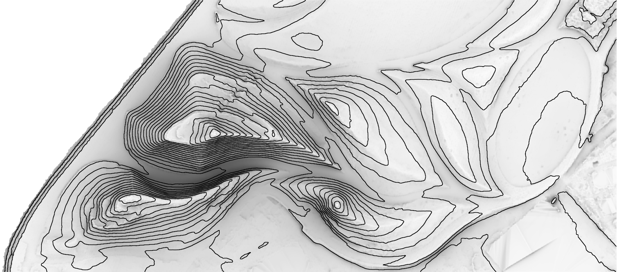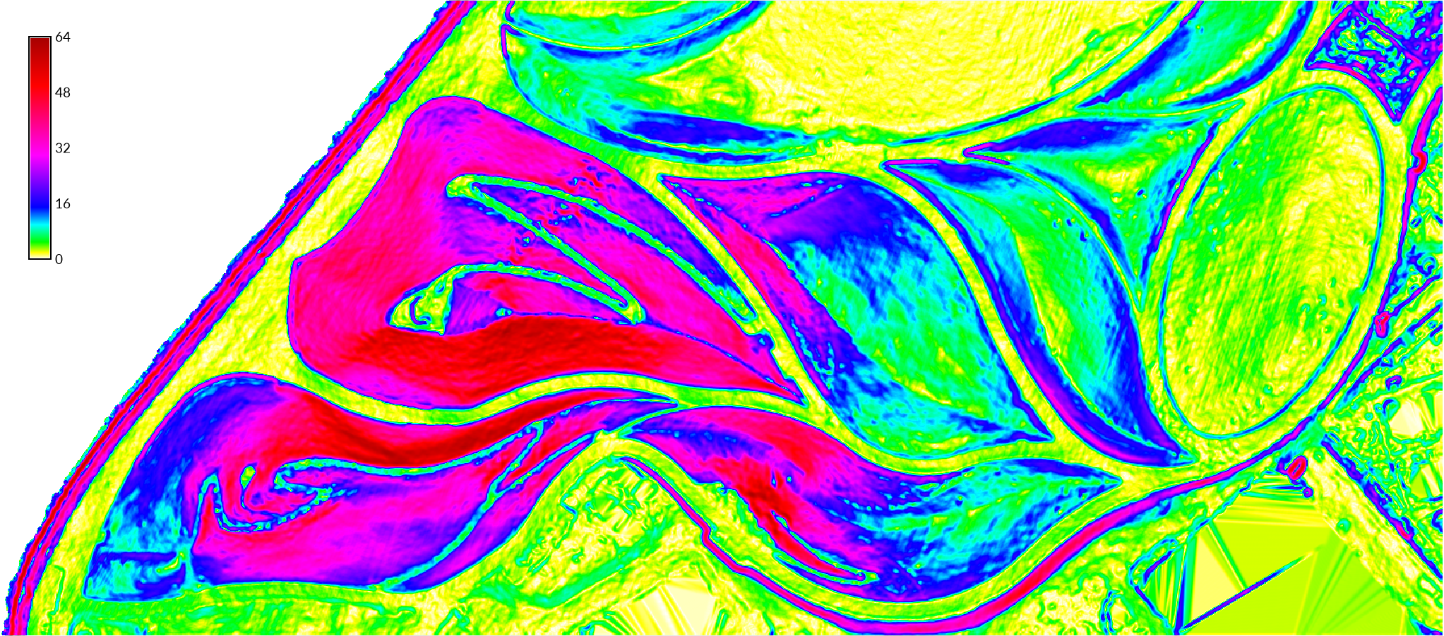
Slope

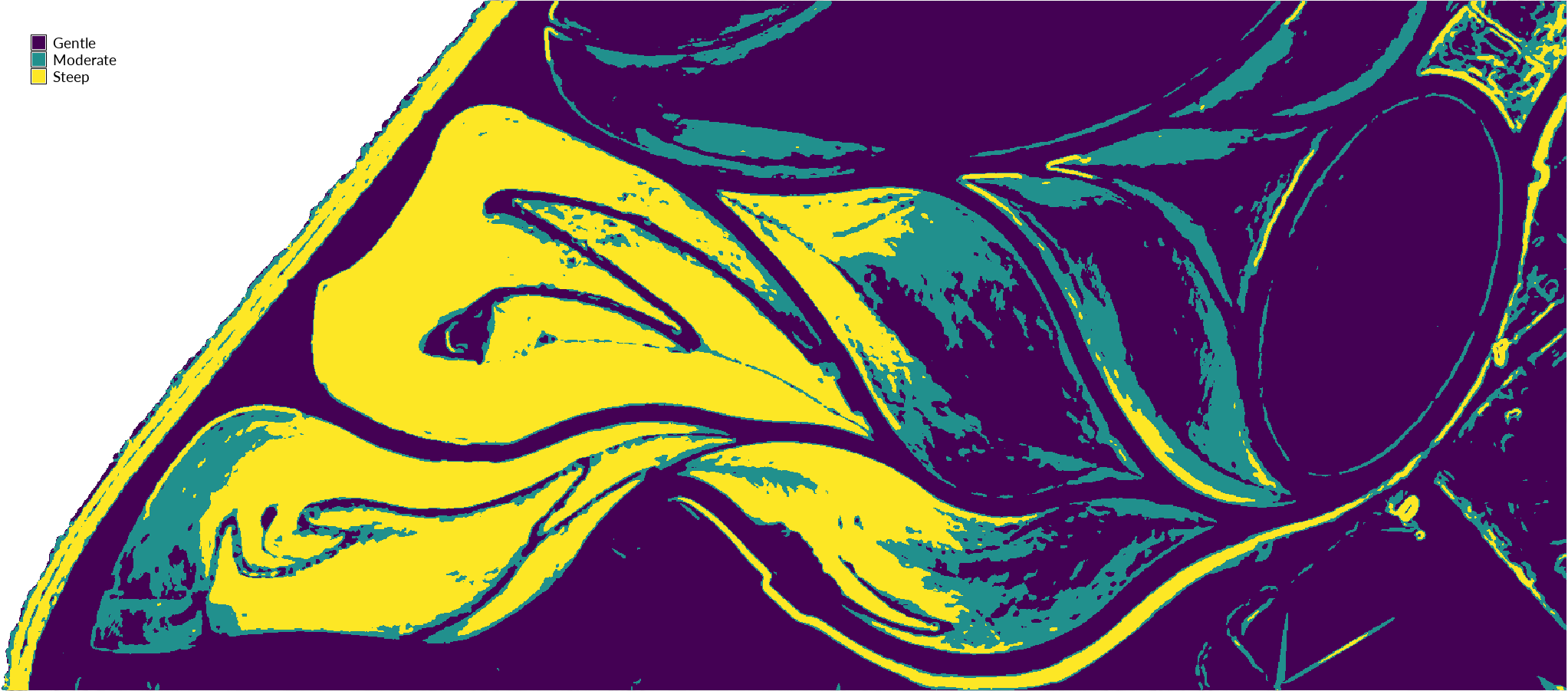
Compute slope in degrees from the smoothed digital elevation model with the module r.slope.aspect and then add a legend. Create a categorized slope map with gentle, moderate, and steep slope categories. Reclassify the continuous slope data into discrete classes using the module r.reclass with the following values entered directly in the required tab:

0 thru 10 = 1
11 thru 20 = 2
21 thru 90 = 3

Then set a category for each class using the module r.category with the following values entered directly into the define tab:

1|Gentle
2|Moderate
3|Steep

Set the color table with the module r.colors and add a legend.

r.slope.aspect -e elevation=elevation slope=slope format=degrees
d.legend raster=slope at=60,95,2,3.5 font=Lato-Regular fontsize=14
r.reclass input=slope output=slope_classes
r.category map=slope_classes separator=pipe
r.colors map=slope_classes color=viridis
d.legend -c raster=slope_classes at=85,95,2,3.5 font=Lato-Regular fontsize=14

Slope

Categorized Slope